Lecture 4: Image Representation Code
Contents
![]()
Lecture 4: Image Representation Code #
#@title
from ipywidgets import widgets
out1 = widgets.Output()
with out1:
  from IPython.display import YouTubeVideo
  video = YouTubeVideo(id=f"PyoJdMrUMqI", width=854, height=480, fs=1, rel=0)
  print("Video available at https://youtube.com/watch?v=" + video.id)
  display(video)
display(out1)
#@title
from IPython import display as IPyDisplay
IPyDisplay.HTML(
    f"""
  <div>
    <a href= "https://github.com/DL4CV-NPTEL/Deep-Learning-For-Computer-Vision/blob/main/Slides/Week_1/DL4CV_Week01_Part04.pdf" target="_blank">
    <img src="https://github.com/DL4CV-NPTEL/Deep-Learning-For-Computer-Vision/blob/main/Data/Slides_Logo.png?raw=1"
  alt="button link to Airtable" style="width:200px"></a>
    </div>""" )
Image as a Matrix#
Import Libraries
from matplotlib import pyplot as plt
import numpy as np
import skimage
from skimage import io
Read 2 images from URL using skimage.
First image is RGB image and second one is the grayscale version
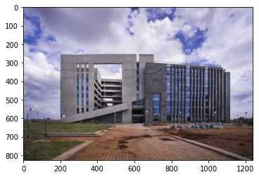
img = io.imread('https://iith.ac.in/assets/images/towers/tower2.jpg')
img_gray = io.imread('https://iith.ac.in/assets/images/towers/tower2.jpg',as_gray = True)
plt.imshow(img)
<matplotlib.image.AxesImage at 0x7fd4d6eb3a10>
Print image as a matrix
img
array([[[123, 126, 177],
        [123, 126, 177],
        [123, 126, 177],
        ...,
        [173, 172, 212],
        [170, 169, 209],
        [167, 166, 206]],

       [[123, 126, 177],
        [123, 126, 177],
        [123, 126, 177],
        ...,
        [172, 171, 211],
        [169, 168, 208],
        [164, 163, 203]],

       [[124, 127, 178],
        [124, 127, 178],
        [124, 127, 178],
        ...,
        [171, 170, 210],
        [168, 167, 207],
        [160, 159, 199]],

       ...,

       [[ 43,  45,  32],
        [ 53,  55,  42],
        [ 54,  56,  43],
        ...,
        [ 45,  40,  36],
        [ 41,  36,  32],
        [ 44,  39,  35]],

       [[ 43,  45,  32],
        [ 53,  55,  42],
        [ 54,  56,  43],
        ...,
        [ 64,  59,  55],
        [ 60,  55,  51],
        [ 51,  46,  42]],

       [[ 43,  45,  32],
        [ 53,  55,  42],
        [ 54,  56,  43],
        ...,
        [ 79,  74,  70],
        [ 77,  72,  68],
        [ 59,  54,  50]]], dtype=uint8)
Check type of image
skimage imread returns an Numpy ndarray
type(img)
numpy.ndarray
Shape of image
Since its an RGB Image, it has 3 channels
img.shape
(827, 1241, 3)
Plot the RGB channels seperately
Remember each channel takes values between 0 and 255 and has the same height and width, so to visualize these channels it is essential that we choose the appropiate color map for the respective channel.
fig, axes = plt.subplots(1, 3,figsize=(15,15))
axes[0].imshow(img[:,:,0],cmap=plt.cm.Reds_r)
axes[1].imshow(img[:,:,1],cmap=plt.cm.Blues_r)
axes[2].imshow(img[:,:,2],cmap=plt.cm.Greens_r)
<matplotlib.image.AxesImage at 0x7fd4d50e1bd0>
Plot the grayscale image.
Remember to use the appropiate color map
plt.imshow(img_gray,cmap = 'gray')
<matplotlib.image.AxesImage at 0x7fd4d501b750>
Print grayscale image as a matrix
Here, the values are normalized between 0 and 1, which is done by skimage while converting RGB image to grayscale. We can always renormalize the values between 0 and 255.
img_gray
array([[0.50603765, 0.50603765, 0.50603765, ..., 0.68665294, 0.67488824,
        0.66312353],
       [0.50603765, 0.50603765, 0.50603765, ..., 0.68273137, 0.67096667,
        0.65135882],
       [0.50995922, 0.50995922, 0.50995922, ..., 0.6788098 , 0.6670451 ,
        0.63567255],
       ...,
       [0.17112824, 0.21034392, 0.21426549, ..., 0.15989843, 0.14421216,
        0.15597686],
       [0.17112824, 0.21034392, 0.21426549, ..., 0.23440824, 0.21872196,
        0.18342784],
       [0.17112824, 0.21034392, 0.21426549, ..., 0.29323176, 0.28538863,
        0.21480039]])
Print shape of grayscale image
Here, there are only 2 dimensions since the third dimesion for Grayscale Image is 1 as opposed to RGB Image which is 3, and is not really required.
img_gray.shape
(827, 1241)
Image as a Function#
Import Libraries
from matplotlib import pyplot as plt
import numpy as np
import skimage
from mpl_toolkits import mplot3d
Get image from skimage.data
skimage.data has a set of saved images for our utiity.
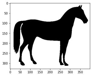
img = skimage.data.horse()
Plot the image of a horse
plt.imshow(img,cmap='gray')
<matplotlib.image.AxesImage at 0x7fd4d4f93e50>
Print shape
img.shape
(328, 400)
Print image as a matrix
Here we notice that the Numpy ndarry is filled with True and False instead of numbers. This is because we are using an binary image that has only 2 values 0 and 1. Storing the values as Boolean instead of int is better in terms of storage for binary images.
img
array([[ True,  True,  True, ...,  True,  True,  True],
       [ True,  True,  True, ...,  True,  True,  True],
       [ True,  True,  True, ...,  True,  True,  True],
       ...,
       [ True,  True,  True, ...,  True,  True,  True],
       [ True,  True,  True, ...,  True,  True,  True],
       [ True,  True,  True, ...,  True,  True,  True]])
Plot the image as a function
fig = plt.figure(figsize=(10,10))
ax = plt.axes(projection='3d')

def f(x,y):
  return img[x,y]

x = np.arange(328)
y = np.arange(400)

X, Y = np.meshgrid(x, y)
Z = f(X, Y)

ax.plot_wireframe(X, Y, Z)
/usr/local/lib/python3.7/dist-packages/mpl_toolkits/mplot3d/art3d.py:304: VisibleDeprecationWarning: Creating an ndarray from ragged nested sequences (which is a list-or-tuple of lists-or-tuples-or ndarrays with different lengths or shapes) is deprecated. If you meant to do this, you must specify 'dtype=object' when creating the ndarray.
  self._segments3d = np.asanyarray(segments)
<mpl_toolkits.mplot3d.art3d.Line3DCollection at 0x7fd4d4ef2510>
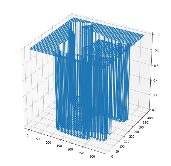
Image Transformations#
Read image
img = skimage.data.camera()
Apply some image transformations and plot
fig, axes = plt.subplots(1, 4,figsize=(15,15))
axes[0].imshow(img,cmap='gray')
axes[1].imshow(img + 40,cmap='gray')
axes[2].imshow(img[::-1],cmap='gray')
axes[3].imshow(img[:,::-1],cmap='gray')
axes[0].title.set_text('Original Image')
axes[1].title.set_text('Image with increased Intensity')
axes[2].title.set_text('Flip Rows')
axes[3].title.set_text('Flip Columns')
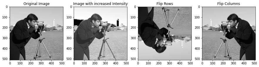
Image processing Operations#
Point operations#
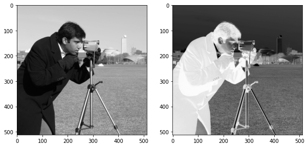
Reversing the contrast#
Read the image
img = skimage.data.camera()
Max and min value of 8-bit image
IMAX = 255
IMIN = 0
Reversing the contrast
img_2 = IMAX - img + IMIN
Plot the images
fig, axes = plt.subplots(1, 2,figsize=(10,10))
axes[0].imshow(img,cmap='gray')
axes[1].imshow(img_2,cmap='gray')
<matplotlib.image.AxesImage at 0x7fd4d47366d0>
Linear contrast stretching#
Read the image
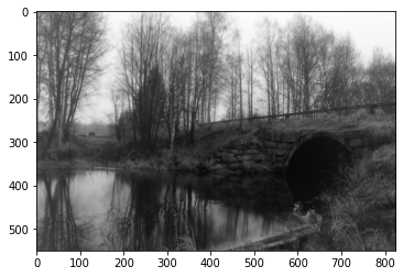
img = io.imread('https://i.pinimg.com/originals/dd/09/c9/dd09c9362c5f18e1185a031f12259332.png')
Print shape
img.shape
(550, 825)
Plot the image
plt.imshow(img,cmap = 'gray')
<matplotlib.image.AxesImage at 0x7fd4d46c4cd0>
Check for min and max value of image
img_min = np.min(img)
img_max = np.max(img)
img_min
61
img_max
250
Apply linear contrast stretching
img_linear_contrast = (img - img_min) * ((IMAX - IMIN)/(img_max - img_min)) + IMIN
fig, axes = plt.subplots(1, 2,figsize=(15,15))
axes[0].imshow(img,cmap='gray')
axes[1].imshow(img_linear_contrast,cmap='gray')
<matplotlib.image.AxesImage at 0x7fd4d45f2c90>
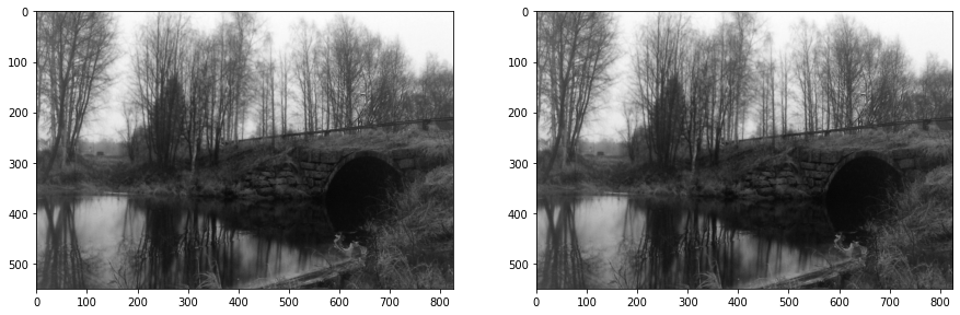
Print min and max value after linear contrast stretching
np.min(img_linear_contrast)
0.0
np.max(img_linear_contrast)
255.00000000000003
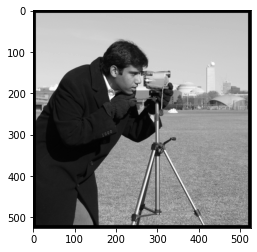
Local operation#
Moving average#
Read image
img = skimage.data.camera()
Define window size
window_size = 15
Compute padding size
Padding means adding some border pixels to the image. In later lectures, we will cover padding in detail and discuss why do we need padding and how to compute it. For now, you can assume padding to be a function of window size to ensure input and output images are of same size. For time being, try odd size window sizes
pad_size = int((window_size - 1)/2)
Initialize an array to store output of moving average
img_mov_avg = np.zeros(shape = img.shape)
Apply padding to image using np.pad
img_padded = np.pad(img,(pad_size,pad_size),constant_values = 0)
Check shape of padded image
img_padded.shape
(526, 526)
Plot the padded image
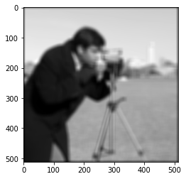
plt.imshow(img_padded,cmap = 'gray')
<matplotlib.image.AxesImage at 0x7fd4d50f3b50>
Compute the moving average
for i in range(img.shape[0]):
  for j in range(img.shape[1]):
    mat = img_padded[i:i+window_size,j:j+window_size]
    img_mov_avg[i,j] = np.mean(mat)
Plot the output image
plt.imshow(img_mov_avg,cmap = 'gray')
<matplotlib.image.AxesImage at 0x7fd4d485d4d0>