Lecture 1: Edge Detection Code
Contents
![]()
Lecture 1: Edge Detection Code #
#@title
from ipywidgets import widgets
out1 = widgets.Output()
with out1:
  from IPython.display import YouTubeVideo
  video = YouTubeVideo(id=f"9r8ph2pb9aw", width=854, height=480, fs=1, rel=0)
  print("Video available at https://youtube.com/watch?v=" + video.id)
  display(video)
display(out1)
#@title
from IPython import display as IPyDisplay
IPyDisplay.HTML(
    f"""
  <div>
    <a href= "https://github.com/DL4CV-NPTEL/Deep-Learning-For-Computer-Vision/blob/main/Slides/Week_2/DL4CV_Week02_Part01.pdf" target="_blank">
    <img src="https://github.com/DL4CV-NPTEL/Deep-Learning-For-Computer-Vision/blob/main/Data/Slides_Logo.png?raw=1"
  alt="button link to Airtable" style="width:200px"></a>
    </div>""" )
SOBEL FILTERS#
The Sobel operator performs a 2-D spatial gradient measurement on an image and so emphasizes regions of high spatial frequency that correspond to edges. Typically it is used to find the approximate absolute gradient magnitude at each point in an input grayscale image.
Implementation#
import numpy as np
import cv2
import argparse
import matplotlib.pyplot as plt
import math
import matplotlib.pyplot as plt
import numpy as np
import warnings
warnings.filterwarnings("ignore")
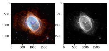
STEP 1 : Converting an image from color to grayscale#
# array representation of image
input_image = plt.imread('https://stsci-opo.org/STScI-01G8GZR18A6CBS9TGJS8JE9CM4.png')
# nx: height, ny: width, nz: colors (RGB)
[nx, ny, nz] = np.shape(input_image)

# Extracting each RGB components
r_img, g_img, b_img = input_image[:, :, 0], input_image[:, :, 1], input_image[:, :, 2]

# Here we are converting the color image to grayscale image by using weights and parameters
gamma = 1.400
# weights for the RGB components respectively
r_const, g_const, b_const = 0.2126, 0.7152, 0.0722
# conversion
grayscale_image = r_const * r_img ** gamma + g_const * g_img ** gamma + b_const * b_img ** gamma

# This command will display the grayscale image alongside the original image
figure1 = plt.figure(1)
ax1, ax2 = figure1.add_subplot(121), figure1.add_subplot(122)
ax1.imshow(input_image)
ax2.imshow(grayscale_image, cmap=plt.get_cmap('gray'))
figure1.show()
STEP2 - Applying the Sobel operator#
Gx is vertical kernel and Gy is the horizontal kernel.
\begin{equation} Gx = \begin{bmatrix} 1.0 & 0.0 & -1.0 \ 2.0 & 0.0 & -2.0 \ 1.0 & 0.0 & -1.0 \end{bmatrix} Gy = \begin{bmatrix} 1.0 & 2.0 & 1.0 \ 0.0 & 0.0 & 0.0 \ -1.0 & -2.0 & -1.0 \end{bmatrix} \end{equation}
# Here we define the matrices associated with the Sobel filter
Gx = np.array([[1.0, 0.0, -1.0], [2.0, 0.0, -2.0], [1.0, 0.0, -1.0]])
Gy = np.array([[1.0, 2.0, 1.0], [0.0, 0.0, 0.0], [-1.0, -2.0, -1.0]])
# shape of the input grayscale image
rows, columns = np.shape(grayscale_image)
# initialize the output images to zeros!
sobel_filtered_image = np.zeros(shape=(rows, columns))
# Convolution operation
for i in range(rows - 2):
for j in range(columns - 2):
gx = np.sum(np.multiply(Gx, grayscale_image[i:i + 3, j:j + 3]))
gy = np.sum(np.multiply(Gy, grayscale_image[i:i + 3, j:j + 3]))
sobel_filtered_image[i + 1, j + 1] = np.sqrt(gx ** 2 + gy ** 2)
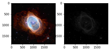
# Display the original image and the Sobel filtered image
figure2 = plt.figure(2)
ax1, ax2 = figure2.add_subplot(121), figure2.add_subplot(122)
ax1.imshow(input_image)
ax2.imshow(sobel_filtered_image, cmap=plt.get_cmap('gray'))
figure2.show()
plt.show()
References :#
https://en.wikipedia.org/wiki/Sobel_operator
https://homepages.inf.ed.ac.uk/rbf/HIPR2/sobel.htm
https://www.geeksforgeeks.org/python-grayscaling-of-images-using-opencv
https://docs.opencv.org/3.4/d2/d2c/tutorial_sobel_derivatives.html
CANNY EDGE DETECTOR#
The Canny edge detector is an edge detection operator that uses a multi-stage algorithm to detect a wide range of edges in images. It was developed by John F. Canny in 1986. Canny also produced a computational theory of edge detection explaining why the technique works.
Algorithm :
Filter image with derivative of Gaussian
Find magnitude and orientation of gradient
Non-maximum supression
Linking and thresholding(hysteresis):
Define two thresholds : low and high
Use the high threshold to start edge curves and the low threshold to continue them.
STEP 1 : apply gaussian filter to reduce the noise from the image#
We can apply gaussian blur to smooth the image. We can do this by convolving the image with Gaussian Kernel. We can have different kenel sizes, sizes depends on the expected blurring effect. Smallest kernel means less visible blur. In our example let’s use 5x5 kernel.
from scipy import ndimage
from scipy.ndimage.filters import convolve
from scipy import misc
import numpy as np
from matplotlib.pyplot import imshow
import numpy as np

def gaussian_kernel(size, sigma=1):
    size = int(size) // 2
    x, y = np.mgrid[-size:size+1, -size:size+1]
    normal = 1 / (2.0 * np.pi * sigma**2)
    g =  np.exp(-((x**2 + y**2) / (2.0*sigma**2))) * normal
    return g
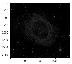
img = plt.imread('https://stsci-opo.org/STScI-01G8GZR18A6CBS9TGJS8JE9CM4.png')
img = cv2.cvtColor(img, cv2.COLOR_RGB2GRAY)
img
array([[0.03096863, 0.02862353, 0.02470196, ..., 0.04528628, 0.04880392,
        0.04447843],
       [0.02493726, 0.03282353, 0.02979608, ..., 0.04281569, 0.02672549,
        0.03109412],
       [0.01451373, 0.01641177, 0.02772941, ..., 0.02789804, 0.02902745,
        0.03267059],
       ...,
       [0.02789804, 0.02397647, 0.02627843, ..., 0.01148628, 0.01451373,
        0.01536471],
       [0.02789804, 0.02397647, 0.02627843, ..., 0.01378824, 0.01451373,
        0.0118902 ],
       [0.04079216, 0.03064706, 0.02627843, ..., 0.01613333, 0.01568628,
        0.01451373]], dtype=float32)
imshow(img, cmap="gray")
<matplotlib.image.AxesImage at 0x7f4704d8c550>

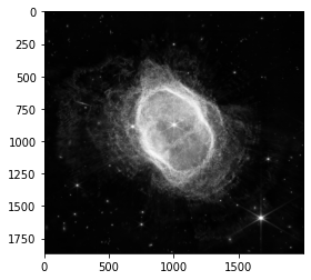
smooth_img = convolve(img, gaussian_kernel(5))
imshow(smooth_img, cmap='gray')
<matplotlib.image.AxesImage at 0x7f470332b250>
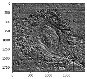
STEP 2 : Find the edge intenity and direction by calculating the gradient of the image using edge detection operators#
For simplicity let’s use the convolve method from scipy
from scipy import ndimage

def sobel_filters(img):
    Kx = np.array([[-1, 0, 1], [-2, 0, 2], [-1, 0, 1]], np.float32)
    Ky = np.array([[1, 2, 1], [0, 0, 0], [-1, -2, -1]], np.float32)

    Ix = ndimage.filters.convolve(img, Kx)
    Iy = ndimage.filters.convolve(img, Ky)

    G = np.hypot(Ix, Iy)
    G = G / G.max() * 255
    theta = np.arctan2(Iy, Ix)

    return (G, theta)
gradientMat, thetaMat = sobel_filters(smooth_img)
gradientMat = gradientMat.astype('uint8')
thetaMat = thetaMat.astype('uint8')
imshow(gradientMat, cmap='gray')
<matplotlib.image.AxesImage at 0x7f470335a250>
imshow(thetaMat, cmap='gray')
<matplotlib.image.AxesImage at 0x7f47032c3210>
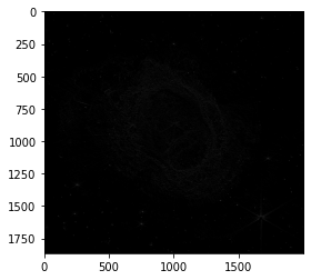
STEP 3 : Non-Maximum Suppression#
def non_max_suppression(img, D):
    M, N = img.shape
    Z = np.zeros((M,N), dtype=np.int32)
    angle = D * 180. / np.pi
    angle[angle < 0] += 180


    for i in range(1,M-1):
        for j in range(1,N-1):
            try:
                q = 255
                r = 255

               #angle 0
                if (0 <= angle[i,j] < 22.5) or (157.5 <= angle[i,j] <= 180):
                    q = img[i, j+1]
                    r = img[i, j-1]
                #angle 45
                elif (22.5 <= angle[i,j] < 67.5):
                    q = img[i+1, j-1]
                    r = img[i-1, j+1]
                #angle 90
                elif (67.5 <= angle[i,j] < 112.5):
                    q = img[i+1, j]
                    r = img[i-1, j]
                #angle 135
                elif (112.5 <= angle[i,j] < 157.5):
                    q = img[i-1, j-1]
                    r = img[i+1, j+1]

                if (img[i,j] >= q) and (img[i,j] >= r):
                    Z[i,j] = img[i,j]
                else:
                    Z[i,j] = 0

            except IndexError as e:
                pass

    return Z
nonMaxImg = non_max_suppression(gradientMat, thetaMat)
imshow(nonMaxImg, cmap='gray')
<matplotlib.image.AxesImage at 0x7f47031f4ad0>
STEP 4 : Linking and Thresholding#
def threshold(img, lowThresholdRatio=0.05, highThresholdRatio=0.09):

    highThreshold = img.max() * highThresholdRatio;
    lowThreshold = highThreshold * lowThresholdRatio;

    M, N = img.shape
    res = np.zeros((M,N), dtype=np.int32)

    weak = np.int32(25)
    strong = np.int32(255)

    strong_i, strong_j = np.where(img >= highThreshold)
    zeros_i, zeros_j = np.where(img < lowThreshold)

    weak_i, weak_j = np.where((img <= highThreshold) & (img >= lowThreshold))

    res[strong_i, strong_j] = strong
    res[weak_i, weak_j] = weak

    return res
thresholdImg = threshold(nonMaxImg)
imshow(thresholdImg, cmap='gray')
<matplotlib.image.AxesImage at 0x7f47031c9b50>

def hysteresis(img):

    M, N = img.shape
    weak = 75 # weak pixel
    strong = 355 #stron pixel

    for i in range(1, M-1):
        for j in range(1, N-1):
            if (img[i,j] == weak):
                try:
                    if ((img[i+1, j-1] == strong) or (img[i+1, j] == strong) or (img[i+1, j+1] == strong)
                        or (img[i, j-1] == strong) or (img[i, j+1] == strong)
                        or (img[i-1, j-1] == strong) or (img[i-1, j] == strong) or (img[i-1, j+1] == strong)):
                        img[i, j] = strong
                    else:
                        img[i, j] = 0
                except IndexError as e:
                    pass

    return img
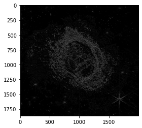
final_img = hysteresis(thresholdImg)
imshow(final_img, cmap='gray')
<matplotlib.image.AxesImage at 0x7f470312ab50>