Lecture 5: Linear Filtering, Correlation, Convolution Code
Contents
![]()
Lecture 5: Linear Filtering, Correlation, Convolution Code #
#@title
from ipywidgets import widgets
out1 = widgets.Output()
with out1:
  from IPython.display import YouTubeVideo
  video = YouTubeVideo(id=f"LiuMJvpSbOU", width=854, height=480, fs=1, rel=0)
  print("Video available at https://youtube.com/watch?v=" + video.id)
  display(video)
display(out1)
#@title
from IPython import display as IPyDisplay
IPyDisplay.HTML(
    f"""
  <div>
    <a href= "https://github.com/DL4CV-NPTEL/Deep-Learning-For-Computer-Vision/blob/main/Slides/Week_1/DL4CV_Week01_Part05.pdf" target="_blank">
    <img src="https://github.com/DL4CV-NPTEL/Deep-Learning-For-Computer-Vision/blob/main/Data/Slides_Logo.png?raw=1"
  alt="button link to Airtable" style="width:200px"></a>
    </div>""" )
Cross- Correlation vs Convolution (using Impulse signal)#
Import libraries
import numpy as np
import matplotlib.pyplot as plt
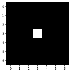
Create a black image with a single white pixel in the middle
img = np.zeros((7,7))
img[3,3] = 1
img
array([[0., 0., 0., 0., 0., 0., 0.],
       [0., 0., 0., 0., 0., 0., 0.],
       [0., 0., 0., 0., 0., 0., 0.],
       [0., 0., 0., 1., 0., 0., 0.],
       [0., 0., 0., 0., 0., 0., 0.],
       [0., 0., 0., 0., 0., 0., 0.],
       [0., 0., 0., 0., 0., 0., 0.]])
Plot the image
plt.imshow(img,cmap='gray')
<matplotlib.image.AxesImage at 0x7f495b460190>
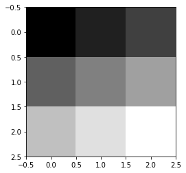
Create a filter that goes from black to white using np.linspace
filter_ = np.linspace(0,1,9).reshape(3,3)
filter_
array([[0.   , 0.125, 0.25 ],
       [0.375, 0.5  , 0.625],
       [0.75 , 0.875, 1.   ]])
Plot the filter
plt.imshow(filter_,cmap='gray')
<matplotlib.image.AxesImage at 0x7f495af3dd50>
Store the filter size and compute value of k
You can obtain k from the following equation \(2*k+1=filter\_size\)
filter_size = filter_.shape[0]
k = int((filter_size - 1)/2)
Cross Correlation#
Empty list to store output image
corr_out = []
Compute cross-correlation
for i in range(k,img.shape[0]-k):
  temp = []
  for j in range(k,img.shape[1]-k):
    mat = img[i-k:i+k+1,j-k:j+k+1]
    temp.append(np.sum(filter_ * mat))
  corr_out.append(temp)
Print shape of output image
corr_out = np.array(corr_out)
corr_out.shape
(5, 5)
Print values of output image
corr_out
array([[0.   , 0.   , 0.   , 0.   , 0.   ],
       [0.   , 1.   , 0.875, 0.75 , 0.   ],
       [0.   , 0.625, 0.5  , 0.375, 0.   ],
       [0.   , 0.25 , 0.125, 0.   , 0.   ],
       [0.   , 0.   , 0.   , 0.   , 0.   ]])
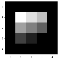
Plot the output image
You will notice that the output is flipped
plt.imshow(corr_out,cmap='gray')
<matplotlib.image.AxesImage at 0x7f495aeb5b90>
Convolution#
Empty list to store output image
conv_out = []
Compute convolution
for i in range(k,img.shape[0]-k):
  temp = []
  for j in range(k,img.shape[1]-k):
    mat = img[i-k:i+k+1,j-k:j+k+1][::-1,::-1]    # You can also use np.flip
    temp.append(np.sum(filter_ * mat))
  conv_out.append(temp)
Print shape of output image
conv_out = np.array(conv_out)
conv_out.shape
(5, 5)
Print values of output image
conv_out
array([[0.   , 0.   , 0.   , 0.   , 0.   ],
       [0.   , 0.   , 0.125, 0.25 , 0.   ],
       [0.   , 0.375, 0.5  , 0.625, 0.   ],
       [0.   , 0.75 , 0.875, 1.   , 0.   ],
       [0.   , 0.   , 0.   , 0.   , 0.   ]])
Plot the output image
You will notice that output is not flipped for convolution
plt.imshow(conv_out,cmap='gray')
<matplotlib.image.AxesImage at 0x7f495ae21410>

Seperable Convolution#
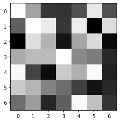
Initialize a 7x7 random image
img = np.random.randint(0,256,(7,7))
img
array([[246, 161,  60,  56,  85, 226,  83],
       [ 98, 248, 228,  62, 230,   9, 217],
       [  8, 217, 176,  28, 163, 213,  19],
       [168, 184, 185, 248, 138, 125,  46],
       [241,  71,  21, 198, 173, 243,  40],
       [198, 179, 131, 112,  68,  26,  47],
       [110, 156,  45,  98, 242, 188,  58]])
Plot the image
plt.imshow(img,cmap='gray')
<matplotlib.image.AxesImage at 0x7f495ae018d0>
2D Gaussian kernel#
Initialize a 2D Gaussian kernel
gaussian_filter_2d =  np.array([[1,2,1],
                              [2,4,2],
                              [1,2,1]])

gaussian_filter_2d = gaussian_filter_2d/16
gaussian_filter_2d
array([[0.0625, 0.125 , 0.0625],
       [0.125 , 0.25  , 0.125 ],
       [0.0625, 0.125 , 0.0625]])
Plot the 2D Gaussian kernel
plt.imshow(gaussian_filter_2d,cmap='gray')
<matplotlib.image.AxesImage at 0x7f495ad719d0>
Store the filter size and compute value of k
You can obtain k from the following equation \(2*k+1=filter\_size\)
filter_size = gaussian_filter_2d.shape[0]
k = int((filter_size - 1)/2)
Empty list to store output image after applying 2D Gaussian kernel
gaussian_2d_out = []
Apply convolution/cross-correlation on the image using 2D Gaussian kernel.
Since the kernel is symmetric, convolutiona as well as cross-correlation will yield the same output
for i in range(k,img.shape[0]-k):
  temp = []
  for j in range(k,img.shape[1]-k):
    mat = img[i-k:i+k+1,j-k:j+k+1]
    temp.append(np.sum(gaussian_filter_2d * mat))
  gaussian_2d_out.append(temp)
Print output image values after applying 2D Gaussian kernel
gaussian_2d_out
[[180.625, 154.125, 113.5, 130.0625, 134.875],
 [173.6875, 172.625, 136.9375, 144.625, 132.1875],
 [154.0, 157.0, 163.9375, 165.75, 135.9375],
 [138.5, 123.5625, 151.375, 156.0625, 124.9375],
 [140.3125, 110.0625, 119.9375, 131.5625, 106.8125]]
1D Gaussian kernels#
Horizontal Gaussian kernel
gaussian_filter_1d_horizontal = np.array([1,2,1])/4
gaussian_filter_1d_horizontal
array([0.25, 0.5 , 0.25])
Vertical Gaussian kernel
gaussian_filter_1d_vertical = np.array([1,2,1])/4
gaussian_filter_1d_vertical
array([0.25, 0.5 , 0.25])
Empty list to store intermediate and final output image after applying the horizontal and vertical kernel
gaussian_1d_out_intermediate = []
gaussian_1d_out = []
Apply the horizontal kernel on the image
Since the kernel is a 1x3 kernel, the number of rows in the output image are not downsampled as opposed to the previous code snippets where both height(rows) and width(columns) were downsampled. The for loop range will be changed accordingly.
for i in range(k,img.shape[0]+1):
  temp = []
  for j in range(k,img.shape[1]-k):
    vec = img[i-k,j-k:j+k+1]    # You can also use np.flip
    temp.append(np.sum(gaussian_filter_1d_horizontal * vec))
  gaussian_1d_out_intermediate.append(temp)
Print the intermediate output after applying the 1D horizontal kernel
As expected, the width of the intermediate output has reduced since the kernel has 3 columns but the height is same as the original image since the kernel has only one row.
gaussian_1d_out_intermediate = np.array(gaussian_1d_out_intermediate)
gaussian_1d_out_intermediate
array([[157.  ,  84.25,  64.25, 113.  , 155.  ],
       [205.5 , 191.5 , 145.5 , 132.75, 116.25],
       [154.5 , 149.25,  98.75, 141.75, 152.  ],
       [180.25, 200.5 , 204.75, 162.25, 108.5 ],
       [101.  ,  77.75, 147.5 , 196.75, 174.75],
       [171.75, 138.25, 105.75,  68.5 ,  41.75],
       [116.75,  86.  , 120.75, 192.5 , 169.  ]])
Apply the vertical kernel on the intermediate image obtained by applying the horizontal kernel in the above snippet
Since the kernel is a 3x1 kernel, the number of columns in the output image are not downsampled after applying the kernel on intermediate image. The for loop range will be changed accordingly.
for i in range(k,gaussian_1d_out_intermediate.shape[0]-k):
  temp = []
  for j in range(k,gaussian_1d_out_intermediate.shape[1]+1):
    vec = gaussian_1d_out_intermediate[i-k:i+k+1,j-k]
    temp.append(np.sum(gaussian_filter_1d_vertical * vec))
  gaussian_1d_out.append(temp)
Print the output obtained by applying 1D kernels
gaussian_1d_out
[[180.625, 154.125, 113.5, 130.0625, 134.875],
 [173.6875, 172.625, 136.9375, 144.625, 132.1875],
 [154.0, 157.0, 163.9375, 165.75, 135.9375],
 [138.5, 123.5625, 151.375, 156.0625, 124.9375],
 [140.3125, 110.0625, 119.9375, 131.5625, 106.8125]]
Print the output which was obtained earlier by applying 2D Gaussian kernel
You will notice that the output is exactly same as the output obtained by applying 1D kernels. This means that the Gaussian kernel is seperable and can be computed by two 1D kernels.
gaussian_2d_out
[[180.625, 154.125, 113.5, 130.0625, 134.875],
 [173.6875, 172.625, 136.9375, 144.625, 132.1875],
 [154.0, 157.0, 163.9375, 165.75, 135.9375],
 [138.5, 123.5625, 151.375, 156.0625, 124.9375],
 [140.3125, 110.0625, 119.9375, 131.5625, 106.8125]]