📺 Lecture video  |  📄 Slides

Watch on YouTube

Week 1, Lecture 4: Image Representation

NPTEL Deep Learning for Computer Vision | Prof. Vineeth N Balasubramanian, IIT Hyderabad

Companion notebook for §1.4 Image Representation.

What you will learn

• Why colour is a 3-vector: how three cone types lead to RGB, and what that means for the image array.

• Read an image both as a matrix of intensities and as a function \(I(x,y)\), and move between the two views.

• Classify every image operation as point, local or global, and reason about the cost of each.

• Apply point operations (contrast reversal, linear stretching, histogram equalization) and see where they run out.

• See why averaging removes noise, motivating local operations (the moving average) and the global Fourier view.

Contents

1. Colour and the eye: why RGB?

2. Image as a matrix

3. Image as a function

4. Image transformations

5. Point / local / global operations (and their cost)

6. Point operations: contrast reversal, linear stretching, histogram equalization

7. Why point operations are limited → denoising by averaging

8. Local operations: the moving average

9. Global operations: the Fourier transform

How to run Runs on Colab or a local Jupyter, CPU only. Every image is bundled with scikit-image, so nothing is downloaded. Run the setup cell first, then go top to bottom.

Review

The previous lecture followed image formation: how light, a lens and a sensor turn a 3D scene into a 2D array of measurements. This lecture starts from that array and asks how to represent and manipulate it, as a matrix and as a function, and how the cost of an operation depends on whether it is point, local or global.

Setup

We rely only on images bundled with scikit-image, so the notebook runs without any network access.

%matplotlib inline
import numpy as np
import matplotlib.pyplot as plt
from matplotlib.patches import Rectangle
from skimage import data, color, util, exposure
from scipy import ndimage

np.random.seed(0)
plt.rcParams['figure.figsize'] = (10, 4)
plt.rcParams['image.cmap']     = 'gray'

1. Colour and the eye: why RGB?

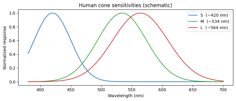
The visible spectrum is continuous (VIBGYOR), yet we encode colour with just three numbers. The reason is biological: the retina has three cone types, Long, Medium and Short wavelength (plus rods for low-light intensity). Any spectrum is collapsed by the eye into three cone responses, so three primaries (R, G, B) are enough to reproduce the same perceived colour.

Fun facts: the M/L cone genes sit on the X-chromosome, so colour-blindness is far more common in men; animals range from 1 cone type (some nocturnal mammals) to 12 (mantis shrimp).

The curves below are a schematic of cone sensitivities (approximate peaks 420 / 534 / 564 nm).

wl = np.linspace(380, 700, 400)
def sens(mu, s):
    y = np.exp(-0.5 * ((wl - mu) / s) ** 2)
    return y / y.max()

plt.figure(figsize=(8, 3.5))
plt.plot(wl, sens(420, 30), color='tab:blue',  label='S  (~420 nm)')
plt.plot(wl, sens(534, 40), color='tab:green', label='M  (~534 nm)')
plt.plot(wl, sens(564, 45), color='tab:red',   label='L  (~564 nm)')
plt.xlabel('Wavelength (nm)'); plt.ylabel('Normalized response')
plt.title('Human cone sensitivities (schematic)')
plt.legend(); plt.tight_layout(); plt.show()

2. Image as a matrix

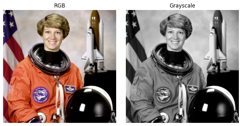
A digital image is a 2D grid of intensity samples. With 8 bits per sample the range is \([0, 255]\) where \(0\) = black and \(255\) = white. A colour image is simply one such matrix per channel, giving an (H, W, 3) array.

rgb  = data.astronaut()        # RGB, uint8, shape (H, W, 3)
gray = color.rgb2gray(rgb)     # grayscale, float in [0, 1], shape (H, W)

print('rgb :', type(rgb).__name__, rgb.dtype,  rgb.shape)
print('gray:', type(gray).__name__, gray.dtype, gray.shape)

rgb : ndarray uint8 (512, 512, 3)
gray: ndarray float64 (512, 512)

.../site-packages/skimage/color/colorconv.py:984: RuntimeWarning: divide by zero encountered in matmul
  return rgb @ coeffs
.../site-packages/skimage/color/colorconv.py:984: RuntimeWarning: overflow encountered in matmul
  return rgb @ coeffs
.../site-packages/skimage/color/colorconv.py:984: RuntimeWarning: invalid value encountered in matmul
  return rgb @ coeffs

fig, ax = plt.subplots(1, 2, figsize=(8, 4))
ax[0].imshow(rgb);             ax[0].set_title('RGB')
ax[1].imshow(gray);            ax[1].set_title('Grayscale')
for a in ax: a.axis('off')
plt.tight_layout(); plt.show()

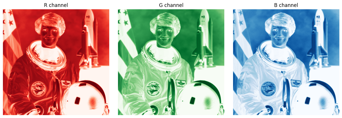
Each colour channel is its own intensity matrix. Plot each with a colormap that matches the channel (R with the reds map, G with greens, B with blues). Bright values mean a strong contribution of that primary.

fig, ax = plt.subplots(1, 3, figsize=(12, 4))
ax[0].imshow(rgb[:, :, 0], cmap='Reds');   ax[0].set_title('R channel')
ax[1].imshow(rgb[:, :, 1], cmap='Greens'); ax[1].set_title('G channel')
ax[2].imshow(rgb[:, :, 2], cmap='Blues');  ax[2].set_title('B channel')
for a in ax: a.axis('off')
plt.tight_layout(); plt.show()

Zooming into an 8x8 patch makes the “matrix of numbers” literal (shown as 0 to 255 intensities):

patch = (gray[180:188, 180:188] * 255).astype(int)
print(patch)

[[ 0  0  7 14 16 11  6 24]
 [ 0  4 12 19 17 14  5 19]
 [ 1  7 12 16 14 11  2 11]
 [ 5  9 14 13 14 14  5  7]
 [ 8  9 10 12 14 12  8  2]
 [ 8  8 12 15 12 13  5  0]
 [ 8  9 10 13 14 13  5  0]
 [13 14 13 16 13  9  9  2]]

3. Image as a function

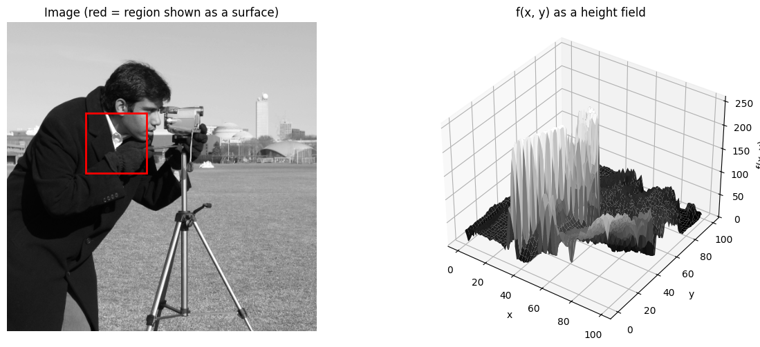
A grayscale image can be modelled as a continuous function \(f : \mathbb{R}^2 \to \mathbb{R}\), where \(f(x, y)\) is the light intensity at position \((x, y)\). A digital image is its discrete counterpart: \(f\) is sampled on a regular integer grid and quantized to a finite bit depth. So the values we actually store are discrete on both axes, position and intensity.

The surface below renders one cropped region (marked in red on the full image). It looks like a smooth sheet only because the plotter shades and interpolates between the samples; the stored data is the grid of pixel values, not a continuous surface.

img_cam = data.camera()                       # 512x512 grayscale test image
r0, c0, h, w = 150, 130, 100, 100             # region to render as a surface
patch = img_cam[r0:r0 + h, c0:c0 + w]
X, Y = np.meshgrid(np.arange(w), np.arange(h))

fig = plt.figure(figsize=(13, 5))
ax1 = fig.add_subplot(121)
ax1.imshow(img_cam)
ax1.add_patch(Rectangle((c0, r0), w, h, fill=False, edgecolor='red', lw=2))
ax1.set_title('Image (red = region shown as a surface)'); ax1.axis('off')

ax2 = fig.add_subplot(122, projection='3d')
ax2.plot_surface(X, Y, patch.astype(float), cmap='gray', linewidth=0)
ax2.set_xlabel('x'); ax2.set_ylabel('y'); ax2.set_zlabel('f(x, y)')
ax2.set_title('f(x, y) as a height field'); ax2.view_init(elev=35, azim=-55)
plt.tight_layout(); plt.show()

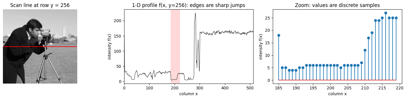
The discreteness is clearest in 1-D. Take a single horizontal row and plot intensity against column: the profile shows edges as sharp jumps, and zooming in reveals that the curve is really a sequence of discrete samples, one per pixel.

row = 256
seg = slice(185, 220)                          # short span to expose individual samples

fig, ax = plt.subplots(1, 3, figsize=(15, 3.5))
ax[0].imshow(img_cam); ax[0].axhline(row, color='red', lw=1.5)
ax[0].set_title(f'Scan line at row y = {row}'); ax[0].axis('off')

ax[1].plot(img_cam[row], color='0.3', lw=1)
ax[1].axvspan(seg.start, seg.stop, color='red', alpha=0.15)
ax[1].set_xlim(0, img_cam.shape[1])
ax[1].set_xlabel('column x'); ax[1].set_ylabel('intensity f(x)')
ax[1].set_title(f'1-D profile f(x, y={row}): edges are sharp jumps')

ax[2].stem(np.arange(seg.start, seg.stop), img_cam[row, seg])
ax[2].set_xlabel('column x'); ax[2].set_ylabel('intensity f(x)')
ax[2].set_title('Zoom: values are discrete samples')
plt.tight_layout(); plt.show()

4. Image transformations

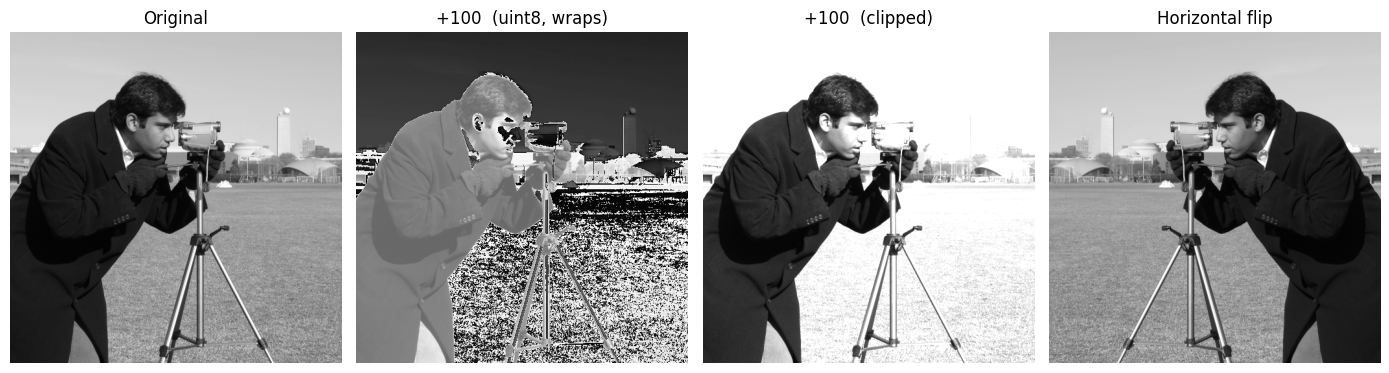
Simple transforms act on intensities or coordinates, e.g. a brightness shift \(\hat I(x, y) = I(x, y) + 20\) or a horizontal flip \(\hat I(x, y) = I(-x, y)\).

Watch the dtype. Images are uint8, so img + 100 overflows: a value like \(200 + 100 = 300\) wraps to \(300 \bmod 256 = 44\), producing dark speckles in bright areas. The fix is to compute in a wider type and saturate with np.clip.

img     = data.camera()
naive   = img + 100                                              # uint8 wraps mod 256
clipped = np.clip(img.astype(np.int16) + 100, 0, 255).astype(np.uint8)
flip    = img[:, ::-1]                                           # I(x, y) -> I(-x, y)

fig, ax = plt.subplots(1, 4, figsize=(14, 4))
for a, im, t in zip(ax, [img, naive, clipped, flip],
                    ['Original', '+100  (uint8, wraps)', '+100  (clipped)', 'Horizontal flip']):
    a.imshow(im); a.set_title(t); a.axis('off')
plt.tight_layout(); plt.show()

5. Point, local and global operations

Image operations are grouped by which inputs determine an output pixel at \((m_0, n_0)\):

Type	Output at \((m_0, n_0)\) depends on	Cost per pixel
Point	the input at the same coordinate	\(O(1)\)
Local	a \(p \times p\) neighbourhood	\(O(p^2)\)
Global	all \(N \times N\) pixels	\(O(N^2)\)

The next sections give a representative operation from each class.

6. Point operations

6.1 Contrast reversal (negative)

\[\hat I(m_0, n_0) = I_{MAX} - I(m_0, n_0) + I_{MIN}\]

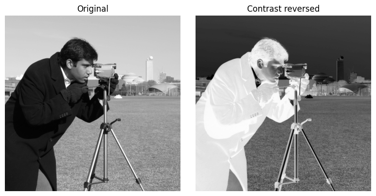
For an 8-bit image (\(I_{MAX}=255,\ I_{MIN}=0\)) this is just 255 - img, which stays in range and is overflow-safe.

img = data.camera()
neg = 255 - img

fig, ax = plt.subplots(1, 2, figsize=(8, 4))
ax[0].imshow(img); ax[0].set_title('Original');          ax[0].axis('off')
ax[1].imshow(neg); ax[1].set_title('Contrast reversed'); ax[1].axis('off')
plt.tight_layout(); plt.show()

6.2 Linear contrast stretching

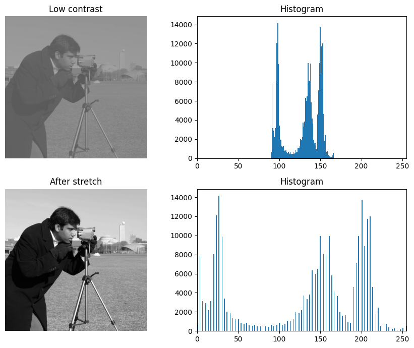
Map the used range \([\min I, \max I]\) onto the full range \([I_{MIN}, I_{MAX}]\):

\[\hat I(m_0, n_0) = \big(I(m_0, n_0) - \min_{x,y} I\big)\cdot \frac{I_{MAX} - I_{MIN}}{\max_{x,y} I - \min_{x,y} I} + I_{MIN}\]

We synthesize a low-contrast image (intensities squeezed into a narrow band) and stretch it back. Note vmin/vmax are fixed in imshow so the washed-out input is shown faithfully instead of being auto-rescaled.

img = data.camera()
low = (img * 0.3 + 90).astype(np.uint8)          # squeeze range into ~[90, 166]
lo, hi = int(low.min()), int(low.max())
stretch = ((low.astype(float) - lo) * (255.0 / (hi - lo))).astype(np.uint8)

print('low-contrast range:', (lo, hi))
print('stretched range   :', (int(stretch.min()), int(stretch.max())))

fig, ax = plt.subplots(2, 2, figsize=(9, 7))
ax[0, 0].imshow(low, vmin=0, vmax=255);     ax[0, 0].set_title('Low contrast'); ax[0, 0].axis('off')
ax[0, 1].hist(low.ravel(), bins=256, range=(0, 255));     ax[0, 1].set_title('Histogram'); ax[0, 1].set_xlim(0, 255)
ax[1, 0].imshow(stretch, vmin=0, vmax=255); ax[1, 0].set_title('After stretch'); ax[1, 0].axis('off')
ax[1, 1].hist(stretch.ravel(), bins=256, range=(0, 255)); ax[1, 1].set_title('Histogram'); ax[1, 1].set_xlim(0, 255)
plt.tight_layout(); plt.show()

low-contrast range: (90, 166)
stretched range   : (0, 255)

6.3 Histogram equalization (homework)

Linear stretching only rescales; it cannot redistribute clustered intensities. Histogram equalization remaps intensities so the output histogram is approximately uniform. The transform is the (scaled) cumulative distribution function:

\[s_k = T(r_k) = (L-1)\sum_{j=0}^{k} p_r(r_j) = \frac{L-1}{MN}\sum_{j=0}^{k} n_j\]

where \(n_j\) is the count of pixels with intensity \(r_j\), \(MN\) the total pixel count, and \(L=256\). Implementing the formula directly (this is exactly the derivation the lecture asks for):

img = data.moon()                                # a genuinely low-contrast image
L = 256
hist = np.bincount(img.ravel(), minlength=L)
cdf  = np.cumsum(hist)
T    = np.round((L - 1) * cdf / cdf[-1]).astype(np.uint8)   # s_k = (L-1) * CDF
eq   = T[img]                                               # apply the mapping

fig, ax = plt.subplots(2, 2, figsize=(9, 7))
ax[0, 0].imshow(img); ax[0, 0].set_title('Original (moon)'); ax[0, 0].axis('off')
ax[0, 1].hist(img.ravel(), bins=256, range=(0, 255)); ax[0, 1].set_title('Histogram'); ax[0, 1].set_xlim(0, 255)
ax[1, 0].imshow(eq);  ax[1, 0].set_title('Equalized');      ax[1, 0].axis('off')
ax[1, 1].hist(eq.ravel(),  bins=256, range=(0, 255)); ax[1, 1].set_title('Histogram'); ax[1, 1].set_xlim(0, 255)
plt.tight_layout(); plt.show()

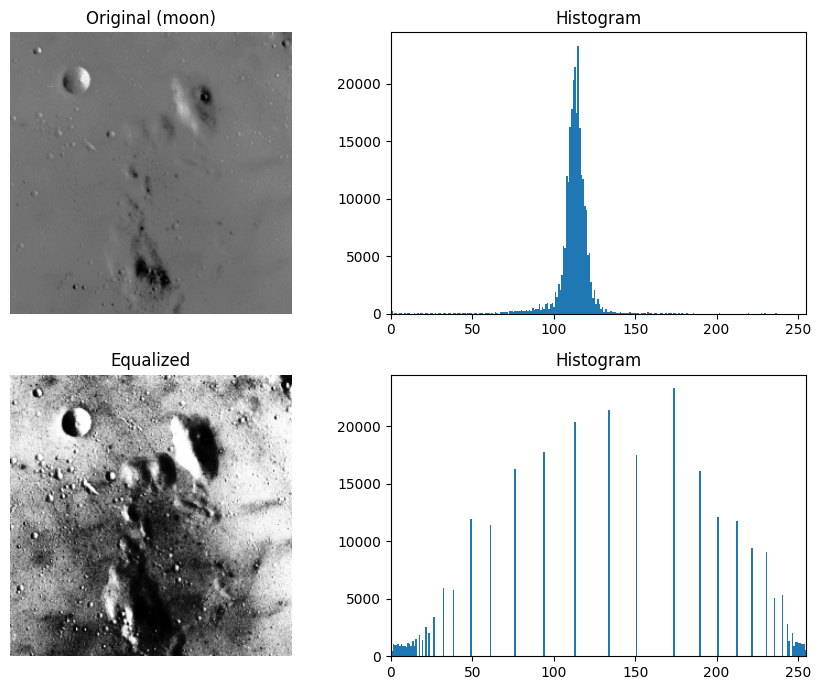
# Cross-check against the library (skimage interpolates, so expect a small difference)
ref = (exposure.equalize_hist(img) * 255).astype(np.uint8)
print('max |manual - skimage|:', int(np.abs(eq.astype(int) - ref.astype(int)).max()))

max |manual - skimage|: 1

7. Why point operations are limited

A single pixel’s value blends many factors (light source, surface geometry and material, sensor noise, colour encoding), so it rarely tells the whole story. For a still scene, one purely point-wise way to fight zero-mean sensor noise is to capture \(N\) frames and average them. The noise std then shrinks as \(\sigma \to \sigma/\sqrt{N}\).

clean = util.img_as_float(data.camera())
sigma = 0.2
noisy = lambda: clean + np.random.normal(0, sigma, clean.shape)

Ns = [1, 4, 16, 64]
fig, ax = plt.subplots(1, len(Ns), figsize=(14, 4))
for a, N in zip(ax, Ns):
    avg  = np.mean([noisy() for _ in range(N)], axis=0)
    meas = float((avg - clean).std())
    a.imshow(np.clip(avg, 0, 1)); a.set_title(f'N = {N}\nnoise std = {meas:.3f}'); a.axis('off')
plt.tight_layout(); plt.show()

print(f'theory  sigma/sqrt(N)  at N=64 : {sigma / np.sqrt(64):.3f}')

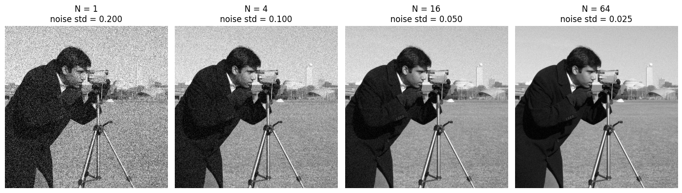
theory  sigma/sqrt(N)  at N=64 : 0.025

If you only have a single image, averaging across frames is impossible, so you instead average over a spatial neighbourhood, which is a local operation.

8. Local operations: the moving average

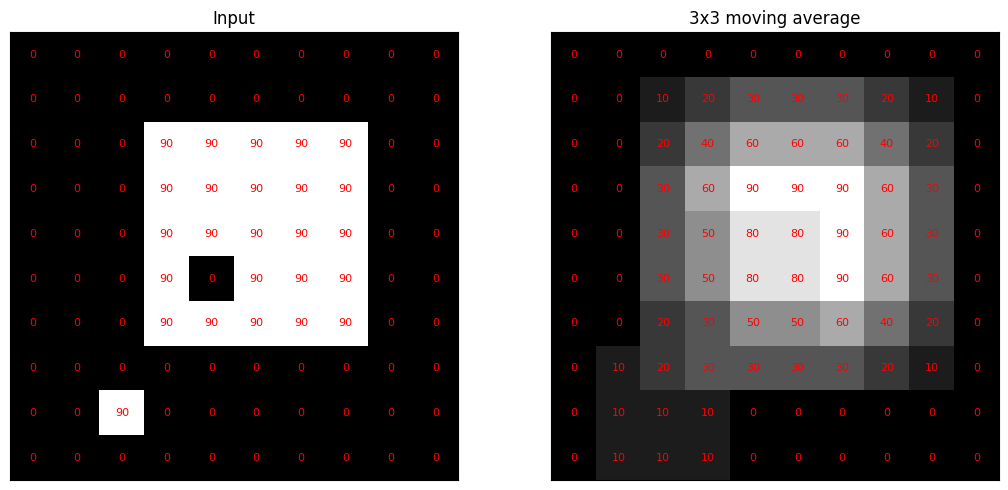
Replace each pixel by the mean of its \(p \times p\) neighbourhood, a simple blur or smoother. First, the worked grid from the lecture: a \(3\times3\) box average turns the sharp 0/90 block into a smoothly ramped output (0, 10, 20, 30, ...).

grid = np.zeros((10, 10))
grid[2:7, 3:8] = 90          # bright block
grid[5, 4]     = 0           # one dark pixel inside it
grid[8, 2]     = 90          # one stray bright pixel
out = ndimage.uniform_filter(grid, size=3, mode='constant')   # 3x3 box mean

fig, ax = plt.subplots(1, 2, figsize=(11, 5))
for a, M, t in zip(ax, [grid, out], ['Input', '3x3 moving average']):
    a.imshow(M, cmap='gray', vmin=0, vmax=90); a.set_title(t)
    for (i, j), v in np.ndenumerate(M):
        a.text(j, i, f'{v:.0f}', ha='center', va='center', color='red', fontsize=8)
    a.set_xticks([]); a.set_yticks([])
plt.tight_layout(); plt.show()

A naive implementation slides the window explicitly, costing \(O(p^2)\) work per pixel. We verify it matches the optimized uniform_filter, then use the fast routine on a real image at several window sizes.

def box_average_naive(img, k):
    p   = k // 2
    pad = np.pad(img, p, mode='constant')        # zero padding keeps output size = input size
    out = np.zeros_like(img, dtype=float)
    for i in range(img.shape[0]):
        for j in range(img.shape[1]):
            out[i, j] = pad[i:i + k, j:j + k].mean()
    return out

crop = data.camera()[:128, :128].astype(float)
slow = box_average_naive(crop, 9)
fast = ndimage.uniform_filter(crop, size=9, mode='constant')
print('naive vs uniform_filter, max diff:', float(np.abs(slow - fast).max()))

naive vs uniform_filter, max diff: 2.8421709430404007e-13

img   = data.camera().astype(float)
sizes = [3, 9, 21]
fig, ax = plt.subplots(1, len(sizes) + 1, figsize=(14, 4))
ax[0].imshow(img); ax[0].set_title('Original'); ax[0].axis('off')
for a, k in zip(ax[1:], sizes):
    a.imshow(ndimage.uniform_filter(img, size=k, mode='reflect'))
    a.set_title(f'{k}x{k} box'); a.axis('off')
plt.tight_layout(); plt.show()

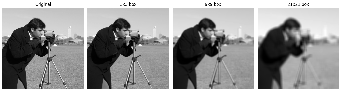
Note: the box filter is separable (a 2D box = two 1D box passes), and integral images give an \(O(1)\)-per-pixel version independent of \(p\). Both are far cheaper than the naive \(O(p^2)\) loop.

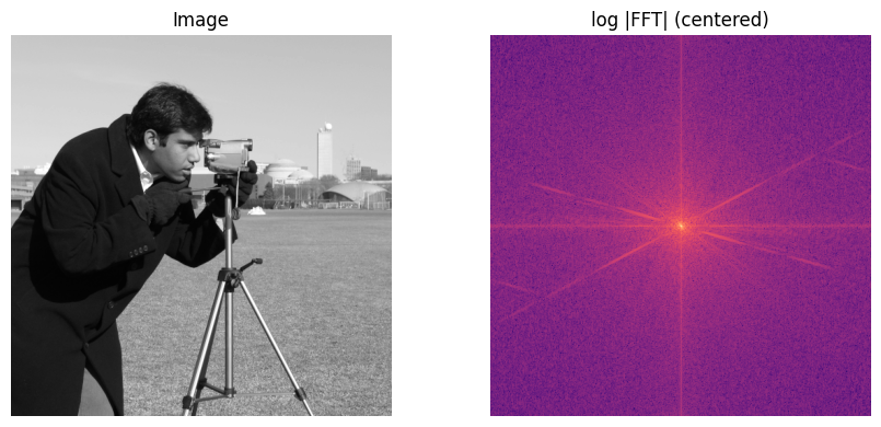
9. Global operations: the Fourier transform

Here every output value depends on all input pixels. The 2D discrete Fourier transform

\[F(u, v) = \sum_{x=0}^{M-1}\sum_{y=0}^{N-1} f(x, y)\, e^{-j 2\pi (ux/M + vy/N)}\]

moves the image to the frequency domain. After centering with fftshift, low frequencies sit at the middle and sharp edges spread energy outward. We revisit frequency-domain filtering later in the course.

img = data.camera().astype(float)
F   = np.fft.fftshift(np.fft.fft2(img))
mag = np.log1p(np.abs(F))                          # log scale for visibility

fig, ax = plt.subplots(1, 2, figsize=(9, 4))
ax[0].imshow(img);            ax[0].set_title('Image');               ax[0].axis('off')
ax[1].imshow(mag, cmap='magma'); ax[1].set_title('log |FFT| (centered)'); ax[1].axis('off')
plt.tight_layout(); plt.show()

10. Explore and verify

Three claims were made above: that the naive moving average really is a moving average, that contrast reversal is its own inverse, and that histogram equalization flattens the cumulative histogram. Rather than take them on trust, we check each one, then vary the window size and watch noise fall while detail blurs.

# Verify the claims made above.
from skimage import exposure, util
from scipy.ndimage import uniform_filter

img = data.camera()

# 1. Our naive box average agrees with the optimized library routine.
k = 5
ours = box_average_naive(img, k)
lib  = uniform_filter(img.astype(float), size=k, mode='reflect')
inner = (slice(k//2, -(k//2)), slice(k//2, -(k//2)))
assert np.allclose(ours[inner], lib[inner], atol=1e-6), 'box average disagrees'

# 2. Contrast reversal is its own inverse: negate twice, get the original back.
assert np.array_equal(255 - (255 - img), img), 'contrast reversal is not an involution'

# 3. Histogram equalization makes the cumulative histogram close to a straight line.
eq = exposure.equalize_hist(img)
cdf = np.cumsum(np.histogram(eq, bins=256, range=(0, 1))[0]) / eq.size
straight = np.linspace(0, 1, 256)
assert np.abs(cdf - straight).max() < 0.06, 'equalized CDF is not close to linear'

print('all three checks passed')
print(f'  box average max |ours - library| = {np.abs(ours[inner] - lib[inner]).max():.2e}')
print(f'  equalized CDF max deviation from a straight line = {np.abs(cdf - straight).max():.3f}')

all three checks passed
  box average max |ours - library| = 5.97e-13
  equalized CDF max deviation from a straight line = 0.017

# Static sweep: what does the window size actually buy, and cost?
noisy = util.random_noise(data.camera(), mode='gaussian', var=0.01, rng=0)

fig, ax = plt.subplots(1, 5, figsize=(15, 3.2))
show_pair = [1, 3, 7, 15, 31]
for a, k in zip(ax, show_pair):
    out = uniform_filter(noisy, size=k, mode='reflect') if k > 1 else noisy
    err = np.sqrt(np.mean((out - data.camera() / 255.0) ** 2))
    a.imshow(out, cmap='gray'); a.set_axis_off()
    a.set_title(f'k = {k}\nRMSE {err:.3f}', fontsize=9)
fig.suptitle('Moving average: noise falls, then detail goes with it', y=1.02)
plt.tight_layout(); plt.show()

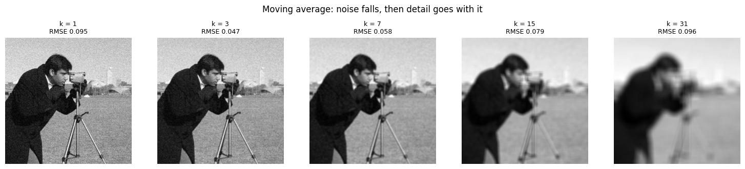
Now the same thing under your control. Drag the slider and watch what changes.

# Live: drag k and watch the trade-off directly.
from ipywidgets import interact, IntSlider

def smooth(k=5):
    out = uniform_filter(noisy, size=k, mode='reflect') if k > 1 else noisy
    rmse = np.sqrt(np.mean((out - data.camera() / 255.0) ** 2))
    fig, a = plt.subplots(figsize=(4.4, 4.4))
    a.imshow(out, cmap='gray'); a.set_axis_off()
    a.set_title(f'window k = {k}   RMSE = {rmse:.3f}')
    plt.show()

interact(smooth, k=IntSlider(min=1, max=41, step=2, value=5, description='window k'));

---

Key takeaways

Concept	Key takeaway
RGB colour	Matches the three cone types (L, M, S) in human vision, so three primaries suffice to reproduce perceived colour
Image as a matrix	uint8 array of shape (H, W) or (H, W, 3); values run 0 (black) to 255 (white), one matrix per channel
Image as a function	\(f : \mathbb{R}^2 \to \mathbb{R}\) gives intensity at \((x, y)\); a digital image is this function sampled on a grid and quantized, so the stored values are discrete on both axes
Transformations	Point-wise intensity or coordinate maps, e.g. \(\hat I = I + b\) (brightness) and \(\hat I(x, y) = I(-x, y)\) (flip); compute in a wider type and clip to avoid uint8 overflow
Point operations	Output depends only on the same pixel; \(O(1)\) per pixel. Examples: contrast reversal \(I_{MAX} - I + I_{MIN}\), linear stretching, histogram equalization (transform = scaled CDF)
Local operations	Output depends on a \(p \times p\) neighbourhood; \(O(p^2)\) per pixel naively. Example: moving average / box filter (low-pass smoothing)
Global operations	Output depends on all \(N \times N\) pixels; \(O(N^2)\) per value. Example: the 2D Fourier transform (centre = low frequencies, edges = high)

Why point operations are limited: a single pixel mixes lighting, geometry, sensor noise and colour, so averaging \(N\) frames of a still scene cuts zero-mean noise as \(\sigma / \sqrt{N}\); with only one image you instead average spatially, which is a local operation.

Further reading: Szeliski, Computer Vision: Algorithms and Applications, Chapter 3.1
Homework: Derive the histogram equalization formula from first principles (PDF/CDF transformation).

Exercises

1. Histogram equalization by hand. Compute the histogram and cumulative histogram of camera() yourself, apply \(\hat I = I_{MAX}\,c\), and compare your result against skimage.exposure.equalize_hist. Where do the two differ, and why?

2. Cost of the three operation classes. For a \(512\times512\) image, count the multiply-adds needed for a point operation, a \(5\times5\) moving average, and a full 2D DFT. At what kernel size does the local operation become more expensive than the global one?

3. Robust contrast stretching. Write a linear stretch that maps the 1st and 99th percentiles to 0 and 255 instead of the min and max. Show an image where this is visibly more robust, and explain what the min/max version is sensitive to.

4. Two ways to grayscale. Convert astronaut() to grayscale twice: once as a plain channel mean, once with the luminance weights \((0.2126, 0.7152, 0.0722)\). Display the difference image and explain which is perceptually correct.