Week 3, Lecture 7: Regularization and L2 Weight Decay

Week 3, Lecture 7: Regularization and L2 Weight Decay#

NPTEL Deep Learning for Computer Vision | Prof. Vineeth N Balasubramanian, IIT Hyderabad

Companion notebook for §3.4 Regularization in Neural Networks.

Overfitting is when a model memorizes the training data (noise and all) instead of learning the underlying rule. Regularization biases learning toward simpler hypotheses that generalize. This notebook makes the idea concrete, from the “guess my rule” intuition all the way to the eigen-analysis of L2.

What you will learn

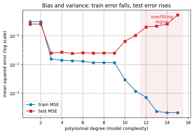
Overfitting made visible: fit polynomials of growing degree to a few noisy points and watch train error fall to zero while test error climbs (the classic bias-variance picture).
Lp norm geometry: draw the unit balls $\lVert w\rVert_p = 1$ and see why small $p$ prefers sparse weights and large $p$ prefers balanced ones.
L2 weight decay: add $\frac{\alpha}{2}\lVert w\rVert^2$ to the loss, get the shrinking update $w_{t+1} = w_t - \eta\nabla L - \eta\alpha w_t$, and watch the overfit curve smooth out.
The eigen-analysis: compute $\tilde w = (H + \alpha I)^{-1} H w^*$ directly and read off why L2 keeps high-curvature directions and discards low-curvature ones.

How to run Everything is tiny and runs in seconds on Colab CPU or GPU (no GPU needed). Run the setup cell first, then go top to bottom. There are 4 interactive widgets; move the sliders to explore.

Contents

What is regularization? The “guess my rule” intuition
Overfitting made visible
Lp norm geometry: why the choice of norm matters
L2 regularization = weight decay
The eigen-analysis: which directions does L2 keep?

Review#

The previous lecture worked through batch, stochastic and mini-batch gradient descent, learning rate schedules, and the adaptive optimizers Adagrad, RMSProp and Adam. All of them fit the training data better. This lecture asks the opposite question: how to stop a model fitting it too well.

Setup#

# Run this cell first. Works on Colab (CPU or GPU) and local Jupyter.
import sys, subprocess
# ipywidgets ships with Colab; install only if it is missing.
try:
    import ipywidgets  # noqa: F401
except ImportError:
    subprocess.run([sys.executable, "-m", "pip", "install", "-q", "ipywidgets"])

import numpy as np
import torch
import torch.nn as nn
import torch.nn.functional as F
import matplotlib.pyplot as plt
from ipywidgets import interact, interactive, FloatSlider, IntSlider, Dropdown, Checkbox, fixed
%matplotlib inline

# Reproducibility
torch.manual_seed(0)
np.random.seed(0)

# Use a GPU if one is available, otherwise CPU. Every demo here is tiny and
# runs in seconds on CPU, so no GPU is required.
device = torch.device("cuda" if torch.cuda.is_available() else "cpu")

plt.rcParams["figure.figsize"] = (7, 4.5)
plt.rcParams["axes.grid"] = True
plt.rcParams["axes.axisbelow"] = True

print("PyTorch", torch.__version__, "| device:", device)

PyTorch 2.8.0 | device: cpu

0. What is regularization? The “guess my rule” intuition#

From the slide, here is a rule that some number triples satisfy:

triple	verdict
1 2 3	satisfies
4 5 6	satisfies
7 8 9	satisfies
9 2 31	does not satisfy

Many rules are consistent with this evidence:

“three consecutive single digits”
“three consecutive integers”
“three numbers in ascending order”
“three numbers whose sum is less than 25”
… and infinitely many more contrived ones.

Every one of these fits the given data perfectly, yet they disagree wildly on new inputs. Machine learning has the same problem: many hypotheses fit the training set, but most generalize badly.

Regularization is any method that biases learning toward the simpler hypotheses, so the model generalizes instead of memorizing (it avoids overfitting to the training data).

The rest of the notebook makes “simpler” precise and shows one concrete recipe: L2 weight decay.

1. Overfitting made visible#

We fit polynomial regression to 15 noisy samples of a smooth true function $f(x) = \sin(\pi x)$.

A degree-$d$ polynomial is just a linear model on polynomial features: $$\hat y = w_0 + w_1 x + w_2 x^2 + \cdots + w_d x^d = \phi(x)^\top w, \qquad \phi(x) = [1, x, x^2, \ldots, x^d].$$ Stacking $\phi(x)$ for every sample gives the **Vandermonde** feature matrix $\Phi$. We build $\Phi$ from scratch (by repeated multiplication, which stays exact for negative $x$), standardize the columns for numerical stability, then solve the least-squares fit with torch.linalg.pinv.

As the degree grows the model gains capacity: it can bend to pass through every noisy point. Watch the train error fall toward zero while the test error (on fresh points) rises. That growing gap is overfitting.

# ----- section 1 setup: data and the from-scratch polynomial machinery -----
torch.manual_seed(0)

def true_f(x):
    "The smooth rule we are trying to recover."
    return torch.sin(np.pi * x)

# 15 noisy training points, plus a fresh noisy test set to measure generalization.
N_TRAIN = 15
NOISE = 0.15
x_train = torch.linspace(-1.0, 1.0, N_TRAIN, device=device)
y_train = true_f(x_train) + NOISE * torch.randn(N_TRAIN, device=device)

x_test = torch.empty(80, device=device).uniform_(-1.0, 1.0)
y_test = true_f(x_test) + NOISE * torch.randn(80, device=device)

# A dense grid, only for drawing smooth fitted curves.
x_grid = torch.linspace(-1.0, 1.0, 300, device=device)

def vandermonde(x, degree):
    "Build [1, x, x^2, ..., x^degree] by repeated multiplication. Shape (len(x), degree+1)."
    x = x.reshape(-1, 1)
    cols = [torch.ones_like(x)]
    for _ in range(degree):
        cols.append(cols[-1] * x)
    return torch.cat(cols, dim=1)

def design_matrix(x, degree, stats=None):
    """Vandermonde with standardized columns (column 0 stays the bias of 1s).
    Standardizing keeps high powers on a comparable scale so the linear solve is
    well behaved. Pass stats=(mean, std) to reuse the training scaling."""
    Phi = vandermonde(x, degree)
    if stats is None:
        mean = Phi.mean(0).clone(); mean[0] = 0.0
        std = Phi.std(0).clone();   std[0] = 1.0
        std = torch.where(std < 1e-8, torch.ones_like(std), std)
        stats = (mean, std)
    mean, std = stats
    return (Phi - mean) / std, stats

def fit_poly(degree):
    """Least-squares fit of a degree-d polynomial. pinv gives the minimum-norm
    least-squares solution and stays robust for any degree. Returns weights,
    the train scaling, and the train and test MSE."""
    Phi_tr, stats = design_matrix(x_train, degree)
    w = torch.linalg.pinv(Phi_tr) @ y_train
    Phi_te, _ = design_matrix(x_test, degree, stats)
    train_mse = torch.mean((Phi_tr @ w - y_train) ** 2).item()
    test_mse = torch.mean((Phi_te @ w - y_test) ** 2).item()
    return w, stats, train_mse, test_mse

print("train points:", N_TRAIN, "| test points:", x_test.numel(), "| device:", device)

train points: 15 | test points: 80 | device: cpu

# Train and test error as the polynomial degree grows: the bias-variance curve.
degrees = list(range(1, 16))
tr_curve, te_curve = [], []
for d in degrees:
    _, _, tr, te = fit_poly(d)
    tr_curve.append(tr)
    te_curve.append(te)

fig, ax = plt.subplots()
ax.semilogy(degrees, tr_curve, "o-", color="tab:blue", label="train MSE")
ax.semilogy(degrees, te_curve, "s-", color="tab:red", label="test MSE")
ax.axvspan(11.5, 15.5, color="tab:red", alpha=0.08)
ax.text(13.5, max(te_curve), "overfitting\nregion", color="tab:red", ha="center", va="top")
ax.set_xlabel("polynomial degree (model complexity)")
ax.set_ylabel("mean squared error (log scale)")
ax.set_title("Bias and variance: train error falls, test error rises")
ax.legend()
plt.show()

../../_images/d499cf739697761b3dfb2e2252f5779611ac45e7e5aa81f3db03e65eecb14439.png

Widget 1: dial the model complexity#

Slide the polynomial degree. Low degrees underfit (too rigid to follow the curve). High degrees overfit (the red fit wiggles through the noise and shoots past the plot edges), even though the true function is a plain sine. The sweet spot is in between.

def show_polyfit(degree=12):
    w, stats, tr, te = fit_poly(degree)
    Phi_g, _ = design_matrix(x_grid, degree, stats)
    y_hat = (Phi_g @ w).detach().cpu().numpy()
    xg = x_grid.cpu().numpy()

    fig, ax = plt.subplots()
    ax.plot(xg, true_f(x_grid).cpu().numpy(), "k--", label="true f(x) = sin(pi x)")
    ax.scatter(x_train.cpu().numpy(), y_train.cpu().numpy(),
               color="tab:blue", zorder=5, label="noisy train points")
    ax.plot(xg, y_hat, color="tab:red", lw=2, label=f"degree {degree} fit")
    ax.set_ylim(-2.5, 2.5)
    ax.set_xlabel("x"); ax.set_ylabel("y")
    ax.set_title(f"Degree {degree}: train MSE {tr:.3f}, test MSE {te:.3f}")
    ax.legend(loc="upper right")
    plt.show()

interact(show_polyfit, degree=IntSlider(min=1, max=15, step=1, value=12));

2. Lp norm geometry: why the choice of norm matters#

A regularizer penalizes “large” weights, but “large” depends on the norm. The Lp norm is $$\lVert w\rVert_p = \left(\sum_i |w_i|^p\right)^{1/p}.$$

The shape of its unit ball $\{w : \lVert w\rVert_p = 1\}$ tells the whole story. From the slide:

All p-norms penalize larger weights.
$p < 2$ tends to create sparse solutions (lots of exact zeros).
$p > 2$ tends to prefer similar-magnitude weights.

We draw the balls with the superellipse trick: for angle $t$, the point $$\big(\operatorname{sign}(\cos t)\,|\cos t|^{2/p},\ \operatorname{sign}(\sin t)\,|\sin t|^{2/p}\big)$$ satisfies $|w_1|^p + |w_2|^p = 1$ exactly, so it traces the unit ball for any $p > 0$.

def lp_ball(p, n=400):
    "Points on the 2D unit ball ||w||_p = 1 via the superellipse parametrization."
    t = np.linspace(0, 2 * np.pi, n)
    x = np.sign(np.cos(t)) * np.abs(np.cos(t)) ** (2.0 / p)
    y = np.sign(np.sin(t)) * np.abs(np.sin(t)) ** (2.0 / p)
    return x, y

fig, ax = plt.subplots(figsize=(5.6, 5.6))
for p in [0.5, 1.0, 2.0, 4.0]:
    x, y = lp_ball(p)
    ax.plot(x, y, lw=2, label=f"p = {p}")
ax.axhline(0, color="gray", lw=0.8)
ax.axvline(0, color="gray", lw=0.8)
ax.set_aspect("equal")
ax.set_xlabel("w1"); ax.set_ylabel("w2")
ax.set_title("Unit balls ||w||_p = 1 in 2D")
ax.legend(loc="upper right")
plt.show()

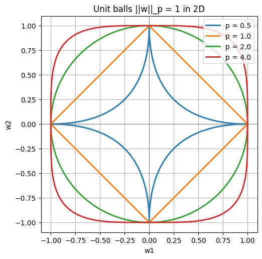
../../_images/f618be476969eea3a0e9398ad86a91903fdb333e02af0eedca7565db2d5f5e5b.png

Reading the picture. Think of learning as inflating a ball from the origin until it first touches the set of weight vectors that fit the data. Where it touches is the solution.

For $p \le 1$ the ball has sharp corners on the axes (the L1 diamond, and the even spikier $p = 0.5$ star). The expanding ball almost always touches first at a corner, where one coordinate is exactly $0$. That is why small $p$ gives sparse solutions.
For $p = 2$ the ball is a smooth circle with no preferred direction: it shrinks weights but rarely drives them to exactly $0$.
For $p > 2$ the ball bulges toward the diagonal, so spreading magnitude evenly across coordinates is “cheapest”: large $p$ prefers balanced weights.

L2 (the circle) is the case we analyze next: smooth, rotationally fair, and easy to differentiate.

def show_lp_ball(p=1.0):
    x, y = lp_ball(p)
    xc, yc = lp_ball(2.0)
    fig, ax = plt.subplots(figsize=(5.6, 5.6))
    ax.plot(xc, yc, color="gray", lw=1.0, ls="--", label="L2 circle (reference)")
    ax.fill(x, y, color="tab:purple", alpha=0.25)
    ax.plot(x, y, color="tab:purple", lw=2, label="unit ball")
    ax.axhline(0, color="gray", lw=0.8)
    ax.axvline(0, color="gray", lw=0.8)
    ax.set_aspect("equal")
    ax.set_xlim(-1.4, 1.4); ax.set_ylim(-1.4, 1.4)
    if p <= 1.0:
        tag = "corners on the axes, sparse friendly"
    elif p > 2.0:
        tag = "bulges to the diagonal, prefers balanced weights"
    else:
        tag = "smooth, no corners"
    ax.set_xlabel("w1"); ax.set_ylabel("w2")
    ax.set_title(f"p = {p:.2f}: {tag}")
    ax.legend(loc="upper right")
    plt.show()

interact(show_lp_ball, p=FloatSlider(min=0.3, max=4.0, step=0.1, value=1.0));

3. L2 regularization = weight decay#

The most common regularizer penalizes the L2 norm of the weights. From the slide, the regularized objective is $$\tilde{L}(w) = L(w) + \frac{\alpha}{2}\lVert w\rVert^2,$$ its gradient is $$\nabla \tilde{L}(w) = \nabla L(w) + \alpha w,$$ and one gradient-descent step becomes $$w_{t+1} = w_t - \eta\,\nabla L(w_t) - \eta\,\alpha\,w_t.$$

The extra term $-\eta\alpha w_t$ nudges every weight toward zero on every step, which is why L2 is called weight decay. Let us confirm from scratch that this is exactly what PyTorch’s weight_decay does.

# The L2 update  w <- w - eta*gradL - eta*alpha*w  should match
# torch.optim.SGD(..., weight_decay=alpha) step for step.
torch.manual_seed(1)
Xr = torch.randn(20, 4, device=device)
yr = torch.randn(20, device=device)
w0 = torch.randn(4, device=device)
eta, alpha = 0.1, 0.3

# (a) from scratch: gradient of the plain loss, then the decayed step by hand.
w_a = w0.clone().requires_grad_(True)
loss_a = 0.5 * torch.mean((Xr @ w_a - yr) ** 2)
loss_a.backward()
w_manual = w_a.detach() - eta * w_a.grad - eta * alpha * w_a.detach()

# (b) idiomatic: let SGD's weight_decay inject the alpha*w term for us.
w_b = w0.clone().requires_grad_(True)
opt = torch.optim.SGD([w_b], lr=eta, weight_decay=alpha)
loss_b = 0.5 * torch.mean((Xr @ w_b - yr) ** 2)
opt.zero_grad(); loss_b.backward(); opt.step()

diff = (w_manual - w_b.detach()).abs().max().item()
print(f"max |manual - SGD(weight_decay)| = {diff:.2e}")
print("They match: weight_decay = alpha IS the -eta*alpha*w shrink term.")

max |manual - SGD(weight_decay)| = 1.19e-07
They match: weight_decay = alpha IS the -eta*alpha*w shrink term.

L2 in action: taming the overfit polynomial#

Now put L2 to work on the degree-12 polynomial from section 1, which badly overfit. Adding $\frac{\alpha}{2}\lVert w\rVert^2$ to the squared-error loss has a closed form, ridge regression: $$\tilde w = (\Phi^\top\Phi + \alpha I)^{-1}\Phi^\top y.$$ Setting $\alpha = 0$ recovers ordinary least squares. As $\alpha$ grows the weights shrink, the curve smooths, and the train-test gap narrows, until too much $\alpha$ underfits everything.

# Fixed high-capacity model (degree 12) that overfits without help.
RIDGE_DEGREE = 12
Phi_tr_r, ridge_stats = design_matrix(x_train, RIDGE_DEGREE)
Phi_te_r, _ = design_matrix(x_test, RIDGE_DEGREE, ridge_stats)
eye_r = torch.eye(RIDGE_DEGREE + 1, device=device)

def fit_ridge(alpha):
    "Closed-form ridge solution for a given alpha (penalizes every weight)."
    A = Phi_tr_r.T @ Phi_tr_r + alpha * eye_r
    w = torch.linalg.solve(A, Phi_tr_r.T @ y_train)
    tr = torch.mean((Phi_tr_r @ w - y_train) ** 2).item()
    te = torch.mean((Phi_te_r @ w - y_test) ** 2).item()
    return w, tr, te

def show_ridge(log_alpha=-2.0):
    alpha = 10.0 ** log_alpha
    w, tr, te = fit_ridge(alpha)
    Phi_g, _ = design_matrix(x_grid, RIDGE_DEGREE, ridge_stats)
    y_hat = (Phi_g @ w).detach().cpu().numpy()
    xg = x_grid.cpu().numpy()
    mags = np.abs(w.detach().cpu().numpy())

    fig, (axL, axR) = plt.subplots(1, 2, figsize=(11, 4.2))
    axL.plot(xg, true_f(x_grid).cpu().numpy(), "k--", label="true f")
    axL.scatter(x_train.cpu().numpy(), y_train.cpu().numpy(),
                color="tab:blue", zorder=5, label="train points")
    axL.plot(xg, y_hat, color="tab:green", lw=2, label="ridge fit")
    axL.set_ylim(-2.5, 2.5)
    axL.set_xlabel("x"); axL.set_ylabel("y")
    axL.set_title(f"alpha = {alpha:.1e}: train MSE {tr:.3f}, test MSE {te:.3f}")
    axL.legend(loc="upper right")

    axR.bar(np.arange(len(mags)), mags, color="tab:orange")
    axR.set_ylim(0, 4.0)
    axR.set_xlabel("coefficient index i")
    axR.set_ylabel("|w_i|")
    axR.set_title(f"Weight magnitudes (L2 norm ||w|| = {np.linalg.norm(mags):.2f})")
    plt.show()

interact(show_ridge, log_alpha=FloatSlider(min=-6.0, max=2.0, step=0.5, value=-2.0));

Notice the two effects together: as $\alpha$ increases the orange bars (weight magnitudes) collapse toward zero, and the green curve relaxes from a wild wiggle into a smooth sine-like shape. Very small $\alpha$ leaves huge coefficients (bars shoot past the top of the axis) and the old overfit; very large $\alpha$ crushes every weight and underfits.

4. The eigen-analysis: which directions does L2 keep?#

Why does L2 help? Look near the unregularized optimum $w^*$, where $\nabla L(w^*) = 0$. A second-order Taylor expansion gives $$L(w) \approx L(w^*) + \tfrac{1}{2}(w - w^*)^\top H (w - w^*), \qquad \nabla L(w) = H(w - w^*),$$ with $H$ the Hessian. The regularized optimum $\tilde w$ satisfies $\nabla\tilde L(\tilde w) = H(\tilde w - w^) + \alpha\tilde w = 0$, hence $(H + \alpha I)\tilde w = H w^$, so $$\tilde w = (H + \alpha I)^{-1} H w^*.$$

Diagonalize the symmetric PSD Hessian as $H = Q\Lambda Q^\top$ (with $Q$ orthogonal). In the eigenbasis, each coordinate of $Q^\top w^*$ is scaled by $$\frac{\lambda_i}{\lambda_i + \alpha}.$$

High curvature ($\lambda_i \gg \alpha$): factor $\approx 1$, the direction is kept.
Low curvature ($\lambda_i \ll \alpha$): factor $\approx 0$, the direction is shrunk away.

The effective number of parameters is $\sum_i \frac{\lambda_i}{\lambda_i + \alpha} < n$. In words: L2 rotates $w^*$ into the eigenbasis, shrinks each direction by its own factor, then rotates back, keeping only the well-determined (high-curvature) directions.

We make this concrete with a 2D bowl whose Hessian has eigenvalues $\lambda = [10, 0.5]$: one steep direction and one shallow one.

# A 2D quadratic bowl with a KNOWN, anisotropic Hessian H = Q Lambda Q^T.
# This part is pure analytic linear algebra (no training), so we use numpy.
theta = np.deg2rad(35.0)
Q = np.array([[np.cos(theta), -np.sin(theta)],
              [np.sin(theta),  np.cos(theta)]])
lam = np.array([10.0, 0.5])          # steep (high curvature), shallow (low curvature)
H = Q @ np.diag(lam) @ Q.T
w_star = np.array([3.0, 2.0])        # the unregularized optimum

def w_tilde_direct(a):
    "Regularized optimum via the matrix formula (H + a I)^{-1} H w*."
    return np.linalg.solve(H + a * np.eye(2), H @ w_star)

def w_tilde_eigen(a):
    "Same thing via per-direction scaling lambda_i / (lambda_i + a)."
    c = Q.T @ w_star                 # rotate w* into the eigenbasis
    c_scaled = (lam / (lam + a)) * c
    return Q @ c_scaled              # rotate back

# The matrix inverse and the per-direction scaling must agree.
print("direct :", np.round(w_tilde_direct(1.0), 6))
print("eigen  :", np.round(w_tilde_eigen(1.0), 6))
assert np.allclose(w_tilde_direct(1.0), w_tilde_eigen(1.0))
print("H eigenvalues:", np.round(np.linalg.eigvalsh(H), 4), "(expected 0.5 and 10)")

# Precompute the loss surface and the shrinkage path, so the widget stays fast.
gx = np.linspace(-1.2, 4.2, 160)
gy = np.linspace(-1.2, 3.4, 160)
GX, GY = np.meshgrid(gx, gy)
D0, D1 = GX - w_star[0], GY - w_star[1]
L_grid = 0.5 * (H[0, 0] * D0 ** 2 + 2 * H[0, 1] * D0 * D1 + H[1, 1] * D1 ** 2)

alpha_path = np.logspace(-2, 4, 60)
wt_path = np.array([w_tilde_direct(a) for a in alpha_path])
print("path endpoints:", np.round(wt_path[0], 2), "->", np.round(wt_path[-1], 2))

direct : [2.700053 1.857056]
eigen  : [2.700053 1.857056]
H eigenvalues: [ 0.5 10. ] (expected 0.5 and 10)
path endpoints: [3. 2.] -> [0. 0.]

Widget 4: watch L2 shrink the low-curvature direction#

Slide $\alpha$. At tiny $\alpha$, $\tilde w \approx w^*$. As $\alpha$ grows, $\tilde w$ slides along the gray path toward the origin, but not in a straight line: the shallow (low-curvature) direction collapses first while the steep (high-curvature) direction holds on. The title reports the two scaling factors and the effective parameter count.

def show_eigen(log_alpha=0.0):
    alpha = 10.0 ** log_alpha
    wt = w_tilde_direct(alpha)
    s_hi = lam[0] / (lam[0] + alpha)   # high curvature (lambda = 10)
    s_lo = lam[1] / (lam[1] + alpha)   # low curvature  (lambda = 0.5)
    eff = s_hi + s_lo

    fig, ax = plt.subplots(figsize=(6.4, 5.4))
    ax.contour(GX, GY, L_grid, levels=18, colors="tab:blue", linewidths=0.7, alpha=0.6)
    # eigenvector directions (the axes of the elliptical contours) through w*.
    dirs = [(0, "high curvature", "tab:red"), (1, "low curvature", "tab:green")]
    for k, name, col in dirs:
        d = Q[:, k]
        ax.plot([w_star[0] - 1.2 * d[0], w_star[0] + 1.2 * d[0]],
                [w_star[1] - 1.2 * d[1], w_star[1] + 1.2 * d[1]],
                color=col, lw=1.4, ls=":", label=f"{name} (lambda = {lam[k]:g})")
    ax.plot(wt_path[:, 0], wt_path[:, 1], color="gray", lw=1.2, label="w_tilde path")
    ax.scatter(*w_star, color="black", marker="*", s=110, zorder=6, label="w* (no reg)")
    ax.scatter(0, 0, color="tab:purple", s=45, zorder=6, label="origin")
    ax.scatter(*wt, color="tab:orange", s=95, zorder=7, label="w_tilde (with L2)")
    ax.set_xlim(-1.2, 4.2); ax.set_ylim(-1.2, 3.4)
    ax.set_xlabel("w1"); ax.set_ylabel("w2")
    ax.set_title(f"alpha = {alpha:.2g}: keep hi (x{s_hi:.2f}), shrink lo (x{s_lo:.2f}), "
                 f"eff params = {eff:.2f}")
    ax.legend(loc="upper left", fontsize=8)
    plt.show()

interact(show_eigen, log_alpha=FloatSlider(min=-2.0, max=3.0, step=0.25, value=0.0));

What the widget shows.

At tiny $\alpha$, both factors are near $1$ and $\tilde w \approx w^*$: effectively no regularization.
As $\alpha$ grows, the low-curvature factor $\frac{0.5}{0.5+\alpha}$ drops fast while the high-curvature factor $\frac{10}{10+\alpha}$ stays close to $1$. So $\tilde w$ moves mostly along the shallow direction toward the origin.
The effective parameter count $\sum_i \frac{\lambda_i}{\lambda_i+\alpha}$ falls from $2$ (both directions free) toward $0$ (everything frozen at the origin).

That is the whole message of the slide: L2 does not shrink all weights equally. It keeps the directions the data constrains well (large curvature) and discards the rest.

Key takeaways#

Regularization biases learning toward simpler hypotheses so it generalizes, instead of memorizing the training data (the “guess my rule” problem).
Overfitting is visible: growing the polynomial degree drives train MSE to zero while test MSE climbs. Capacity without a preference for simplicity is dangerous.
Lp geometry: the unit ball’s shape sets the prior. $p \le 1$ has axis corners and gives sparse weights; $p = 2$ is a smooth circle; $p > 2$ prefers balanced weights.
L2 = weight decay: adding $\frac{\alpha}{2}\lVert w\rVert^2$ appends $-\eta\alpha w$ to every SGD step, exactly PyTorch’s weight_decay. It shrinks weights, smooths the fit, and closes the train-test gap.
Eigen-analysis: near $w^*$, $\tilde w = (H + \alpha I)^{-1} H w^*$ scales each eigen-direction by $\frac{\lambda_i}{\lambda_i+\alpha}$. High-curvature directions survive, low-curvature ones vanish, and the effective parameter count is $\sum_i \frac{\lambda_i}{\lambda_i+\alpha} < n$.

Exercises#

In the ridge widget (section 3), hunt for the $\alpha$ that minimizes test MSE. How does its fit compare to the best polynomial degree from section 1? Two different knobs, one shared goal.
Preview of Lecture 8 and 9: adding small Gaussian noise to the inputs of a linear model is equivalent, in expectation, to L2 weight decay on the weights. Try it: add eps * torch.randn_like(x_train) to the inputs before fitting and watch the fit stabilize like ridge. Regularization can come from the data, not only the loss.