📺 Lecture video  |  📄 Slides

Watch on YouTube

Week 2, Lecture 1: Edge Detection

NPTEL Deep Learning for Computer Vision | Prof. Vineeth N Balasubramanian, IIT Hyderabad

Companion notebook for §2.1 Edge Detection.

What you will learn

• Treat an edge as rapid intensity change, and compute derivatives by convolution with finite differences.

• Compare the Prewitt, Sobel and Roberts filters, and read gradient strength and orientation.

• See why noise forces you to smooth first, and use the derivative-of-Gaussian shortcut.

• Find edges with the Laplacian of Gaussian and its zero-crossings.

• Assemble the Canny detector: non-maximum suppression followed by hysteresis thresholding.

Contents

1. An edge is a place of rapid intensity change

2. Derivatives as convolution: finite differences

3. Finite difference filters: Prewitt, Sobel, Roberts

4. The image gradient: strength and orientation

5. Noise, and why we smooth first

6. Derivative theorem of convolution: derivative of Gaussian

7. Second derivative: Laplacian of Gaussian and zero-crossings

8. Non-maximum suppression

9. Hysteresis thresholding

10. The Canny edge detector

11. Beyond Canny: learned edge detection

How to run Runs on Colab or a local Jupyter, CPU only. Every image is bundled with scikit-image, so nothing is downloaded. Run the setup cell first, then go top to bottom.

Review

The earlier lectures built up convolution and linear filtering. Edge detection is the first place those tools pay off as a vision task. The plan is simple to state: an edge is where image intensity changes sharply, so a derivative will be large there, and a derivative of a discrete signal is itself a convolution with a small kernel. The rest of the notebook turns that one idea into a detector that is robust to noise, returns thin one-pixel contours, and links them into connected curves, which is exactly the Canny pipeline.

Setup

Everything uses images bundled with scikit-image, so the notebook runs offline. We apply named kernels with correlate (the kernel slides without being flipped), so the matrices shown in code match the ones on the slides.

%matplotlib inline
import numpy as np
import matplotlib.pyplot as plt
from matplotlib.colors import hsv_to_rgb
from scipy import ndimage as ndi
from skimage import data, util, color

np.random.seed(0)
plt.rcParams['figure.figsize'] = (10, 4)
plt.rcParams['image.cmap']     = 'gray'
plt.rcParams['figure.dpi']     = 85

def load_gray(image):
    # float grayscale image in [0, 1]
    return color.rgb2gray(image) if image.ndim == 3 else util.img_as_float(image)

def show(ax, im, title='', cmap='gray'):
    ax.imshow(im, cmap=cmap); ax.set_title(title); ax.axis('off')

cam = load_gray(data.camera())

1. An edge is a place of rapid intensity change

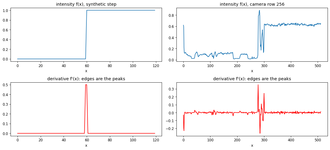
Take a single horizontal scanline through an image and plot intensity against position. A clean edge shows up as a step, and its derivative shows up as a sharp peak whose location marks the edge. So locating edges in 1D reduces to finding extrema of the derivative. The synthetic step on the left makes this exact; the real scanline on the right shows the same structure buried in texture.

# synthetic step edge and a real scanline from the camera image
step = np.concatenate([np.zeros(60), np.ones(60)])
row  = cam[256]                                   # one row through the middle

fig, ax = plt.subplots(2, 2, figsize=(13, 6))
for col, (sig, name) in enumerate([(step, 'synthetic step'), (row, 'camera row 256')]):
    d = np.gradient(sig)                           # discrete derivative
    ax[0, col].plot(sig);  ax[0, col].set_title(f'intensity f(x), {name}'); ax[0, col].set_xlabel('x')
    ax[1, col].plot(d, 'r'); ax[1, col].set_title("derivative f'(x): edges are the peaks"); ax[1, col].set_xlabel('x')
plt.tight_layout(); plt.show()

2. Derivatives as convolution: finite differences

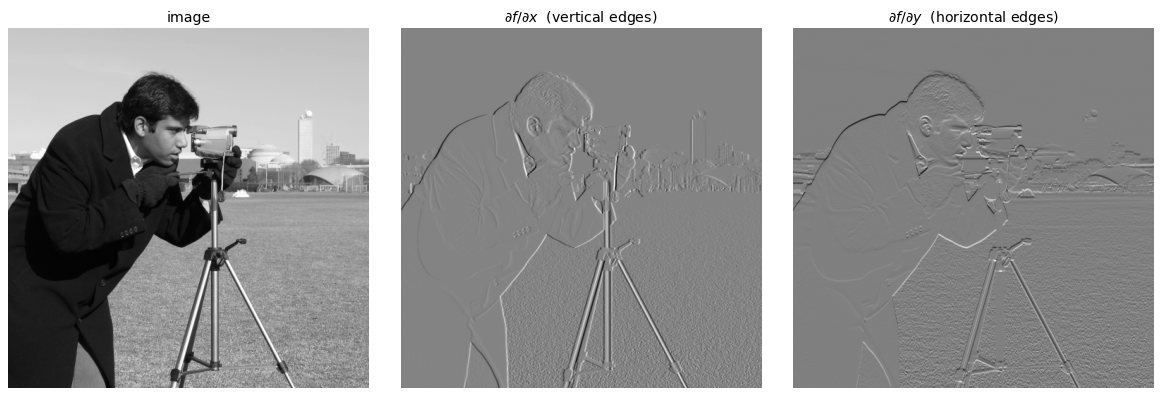
For a discrete image the partial derivative is approximated by a finite difference, \(\partial f/\partial x \approx f(x{+}1, y) - f(x{-}1, y)\) for the central form. That subtraction of neighbouring pixels is a correlation with the 1D kernel \([-1, 0, 1]\), and the vertical kernel \([-1, 0, 1]^\top\) gives \(\partial f/\partial y\). The \(x\) derivative responds to vertical edges and the \(y\) derivative to horizontal edges, which is why each result below highlights one orientation.

kx = np.array([[-1, 0, 1]]) / 2.0                 # central difference along x
ky = kx.T                                          # along y

Ix = ndi.correlate(cam, kx)
Iy = ndi.correlate(cam, ky)

fig, ax = plt.subplots(1, 3, figsize=(14, 4.6))
show(ax[0], cam, 'image')
show(ax[1], Ix, r'$\partial f/\partial x$  (vertical edges)')
show(ax[2], Iy, r'$\partial f/\partial y$  (horizontal edges)')
plt.tight_layout(); plt.show()

3. Finite difference filters: Prewitt, Sobel, Roberts

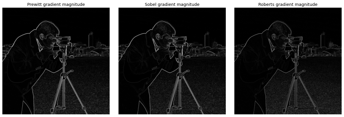
A bare difference is noisy because it uses a single pixel on each side. The classic operators add a small amount of smoothing along the edge. Prewitt averages three rows equally, Sobel weights the centre row by two (a mild Gaussian-like blur), and Roberts is a compact \(2\times 2\) diagonal difference. Sobel is the usual default: cheap, separable, and noticeably steadier than the raw difference.

ops = {
    'Prewitt': (np.array([[-1,0,1],[-1,0,1],[-1,0,1]], float),
                np.array([[-1,-1,-1],[0,0,0],[1,1,1]], float)),
    'Sobel':   (np.array([[-1,0,1],[-2,0,2],[-1,0,1]], float),
                np.array([[-1,-2,-1],[0,0,0],[1,2,1]], float)),
    'Roberts': (np.array([[1,0],[0,-1]], float),
                np.array([[0,1],[-1,0]], float)),
}

def grad_mag(im, kx, ky):
    return np.hypot(ndi.correlate(im, kx), ndi.correlate(im, ky))

fig, ax = plt.subplots(1, 3, figsize=(14, 4.6))
for a, (name, (gx, gy)) in zip(ax, ops.items()):
    show(a, grad_mag(cam, gx, gy), f'{name} gradient magnitude')
plt.tight_layout(); plt.show()

4. The image gradient: strength and orientation

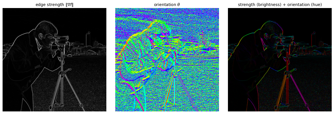
Stacking the two partials gives the gradient \(\nabla f = [\,\partial f/\partial x,\ \partial f/\partial y\,]\), which points in the direction of fastest intensity increase. Its magnitude \(\lVert \nabla f \rVert = \sqrt{f_x^2 + f_y^2}\) is the edge strength, and its angle \(\theta = \operatorname{atan2}(f_y, f_x)\) is the orientation of the edge normal. Below, brightness encodes strength and hue encodes orientation, so edges of different directions take different colours.

gx, gy = ndi.correlate(cam, ops['Sobel'][0]), ndi.correlate(cam, ops['Sobel'][1])
mag    = np.hypot(gx, gy)
theta  = np.arctan2(gy, gx)

# map orientation to hue, strength to value
hsv = np.zeros(cam.shape + (3,))
hsv[..., 0] = (np.degrees(theta) % 180) / 180.0    # hue from edge direction
hsv[..., 1] = 1.0
hsv[..., 2] = mag / mag.max()                       # brightness from edge strength

fig, ax = plt.subplots(1, 3, figsize=(14, 4.6))
show(ax[0], mag, r'edge strength $\|\nabla f\|$')
show(ax[1], theta, r'orientation $\theta$', cmap='hsv')
show(ax[2], hsv_to_rgb(hsv), 'strength (brightness) + orientation (hue)')
plt.tight_layout(); plt.show()

5. Noise, and why we smooth first

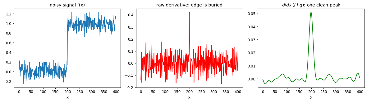
Differentiation amplifies high frequencies, so on a noisy signal the raw derivative is dominated by noise and the edge is lost. The fix is to low-pass first: smooth with a Gaussian \(g\), then differentiate. The edge now appears as a clean peak in \(\frac{d}{dx}(f * g)\). The amount of smoothing trades robustness against localization, a tension the Gaussian scale \(\sigma\) controls.

x = np.linspace(0, 1, 400)
clean = (x > 0.5).astype(float)
noisy = clean + 0.10 * np.random.randn(x.size)
smoothed = ndi.gaussian_filter1d(noisy, 8)

fig, ax = plt.subplots(1, 3, figsize=(14, 4))
ax[0].plot(noisy); ax[0].set_title('noisy signal f(x)')
ax[1].plot(np.gradient(noisy), 'r'); ax[1].set_title("raw derivative: edge is buried")
ax[2].plot(np.gradient(smoothed), 'g'); ax[2].set_title(r'$d/dx\,(f*g)$: one clean peak')
for a in ax: a.set_xlabel('x')
plt.tight_layout(); plt.show()

6. Derivative theorem of convolution: derivative of Gaussian

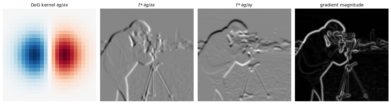
Convolution is associative and differentiation is a convolution, so \(\frac{d}{dx}(f * g) = f * \frac{d}{dx} g\). We can therefore differentiate the Gaussian once, offline, and convolve the image with that single derivative-of-Gaussian (DoG) kernel, smoothing and differentiating in one pass. The \(x\) and \(y\) DoG kernels below sum to zero and act as oriented edge filters; their magnitude is a noise-robust gradient.

def gaussian_2d(size, sigma):
    ax = np.arange(-(size//2), size//2 + 1)
    xx, yy = np.meshgrid(ax, ax)
    g = np.exp(-(xx**2 + yy**2) / (2*sigma**2)) / (2*np.pi*sigma**2)
    return xx, yy, g

s = 4
xx, yy, g = gaussian_2d(25, s)
dog_x = -xx / s**2 * g                              # d/dx of the Gaussian
dog_y = -yy / s**2 * g

# apply DoG directly with scipy's order argument (separable, fast)
Ix = ndi.gaussian_filter(cam, s, order=[0, 1])      # axis 1 = x
Iy = ndi.gaussian_filter(cam, s, order=[1, 0])      # axis 0 = y
dog_mag = np.hypot(Ix, Iy)

fig, ax = plt.subplots(1, 4, figsize=(15, 4))
show(ax[0], dog_x, r'DoG kernel $\partial g/\partial x$', cmap='RdBu')
show(ax[1], Ix, r'$f * \partial g/\partial x$')
show(ax[2], Iy, r'$f * \partial g/\partial y$')
show(ax[3], dog_mag, 'gradient magnitude')
plt.tight_layout(); plt.show()

7. Second derivative: Laplacian of Gaussian and zero-crossings

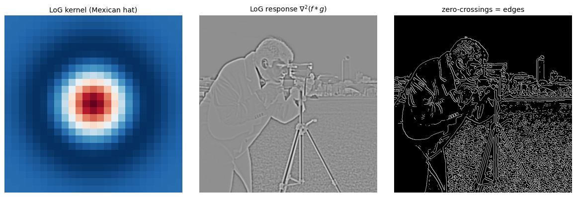
An edge is a peak in the first derivative, which is a zero-crossing in the second derivative. The orientation-free second-order operator is the Laplacian \(\nabla^2 f = f_{xx} + f_{yy}\); combined with Gaussian smoothing it becomes the Laplacian of Gaussian (LoG), the familiar Mexican-hat kernel. Edges are then the points where the LoG response changes sign. This is sharp but more sensitive to noise than the gradient route, visible in the busier zero-crossing map.

s = 2
xx, yy, g = gaussian_2d(25, 4)
log_kernel = (xx**2 + yy**2 - 2*4**2) / 4**4 * g     # Laplacian of Gaussian
log_resp   = ndi.gaussian_laplace(cam, sigma=s)

def zero_crossings(L, rel=0.03):
    zc = np.zeros_like(L, dtype=bool)
    for axis in (0, 1):
        flip = np.diff(np.sign(L), axis=axis) != 0   # sign change along this axis
        pad = [(0, 0), (0, 0)]; pad[axis] = (0, 1)
        zc |= np.pad(flip, pad)
    strength = np.hypot(*np.gradient(L))             # keep only strong crossings
    return zc & (strength > rel * strength.max())

fig, ax = plt.subplots(1, 3, figsize=(14, 4.6))
show(ax[0], log_kernel, 'LoG kernel (Mexican hat)', cmap='RdBu')
show(ax[1], log_resp, r'LoG response $\nabla^2(f*g)$')
show(ax[2], zero_crossings(log_resp), 'zero-crossings = edges')
plt.tight_layout(); plt.show()

8. Non-maximum suppression

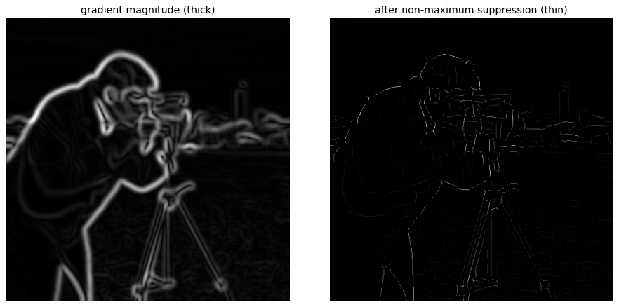
The gradient magnitude is a thick ridge, but a good detector returns one pixel per edge. Non-maximum suppression keeps a pixel only if its magnitude is a local maximum along the gradient direction, comparing against the two neighbours that straddle the edge. We quantize the direction to the nearest of four orientations (0, 45, 90, 135 degrees) and pick neighbours accordingly; an exact version interpolates between pixels. The result is a thin one-pixel ridge.

def non_max_suppression(mag, theta):
    out = np.zeros_like(mag)
    angle = np.degrees(theta) % 180
    p = np.pad(mag, 1)                               # 1-pixel border to avoid edge checks
    M, N = mag.shape
    for i in range(M):
        for j in range(N):
            a, ii, jj = angle[i, j], i + 1, j + 1
            if   a < 22.5 or a >= 157.5: nb = (p[ii, jj+1], p[ii, jj-1])     # horizontal grad
            elif a < 67.5:               nb = (p[ii-1, jj+1], p[ii+1, jj-1]) # diagonal
            elif a < 112.5:              nb = (p[ii-1, jj], p[ii+1, jj])     # vertical grad
            else:                        nb = (p[ii-1, jj-1], p[ii+1, jj+1]) # anti-diagonal
            if mag[i, j] >= max(nb):
                out[i, j] = mag[i, j]
    return out

thin = non_max_suppression(dog_mag, np.arctan2(Iy, Ix))

fig, ax = plt.subplots(1, 2, figsize=(11, 5.2))
show(ax[0], dog_mag, 'gradient magnitude (thick)')
show(ax[1], thin, 'after non-maximum suppression (thin)')
plt.tight_layout(); plt.show()

9. Hysteresis thresholding

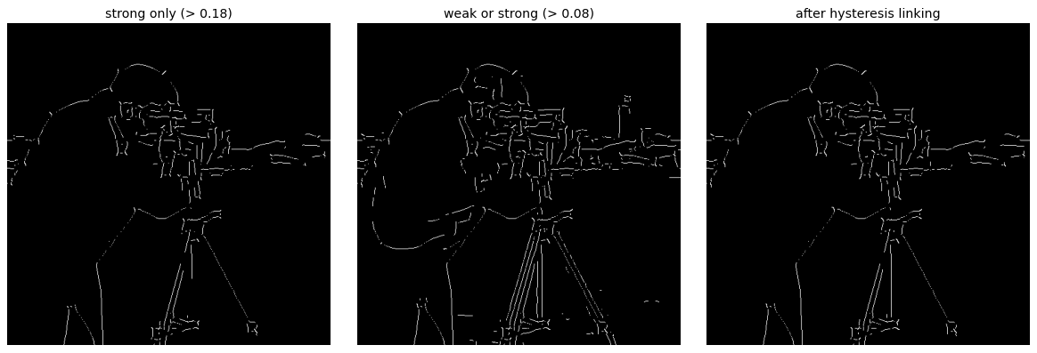
A single threshold either breaks strong edges into dashes or floods the image with noise. Hysteresis uses two: pixels above high are confirmed edges, pixels below low are discarded, and pixels in between are kept only if they connect to a confirmed edge. We implement it by labelling all above-low pixels into connected components and keeping any component that contains an above-high pixel, which links faint but well-connected segments while dropping isolated weak responses.

def hysteresis(mag, low, high):
    strong = mag >= high
    weak   = mag >= low
    labels, n = ndi.label(weak)                      # connected components of weak-or-strong
    keep = np.zeros(n + 1, bool)
    keep[labels[strong]] = True                      # mark components touching a strong pixel
    keep[0] = False
    return keep[labels]

m = thin / thin.max()
low, high = 0.08, 0.18
edges = hysteresis(m, low, high)

fig, ax = plt.subplots(1, 3, figsize=(14, 4.6))
show(ax[0], m >= high, f'strong only (> {high})')
show(ax[1], m >= low, f'weak or strong (> {low})')
show(ax[2], edges, 'after hysteresis linking')
plt.tight_layout(); plt.show()

10. The Canny edge detector

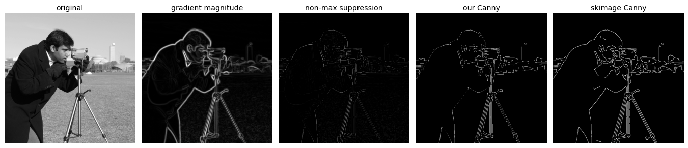
Canny (1986) is exactly the four steps we just built, in order: smooth with a derivative of Gaussian, compute gradient magnitude and orientation, thin by non-maximum suppression, then link with hysteresis. It remains the standard classical detector because it scores well on the three criteria of good detection, good localization, and a single response per edge. Below we assemble our functions into one pass and compare with the reference implementation in scikit-image.

from skimage.feature import canny

def canny_edges(im, sigma=2, low=0.08, high=0.18):
    Ix = ndi.gaussian_filter(im, sigma, order=[0, 1])
    Iy = ndi.gaussian_filter(im, sigma, order=[1, 0])
    mag = np.hypot(Ix, Iy)
    thin = non_max_suppression(mag, np.arctan2(Iy, Ix))
    thin = thin / (thin.max() + 1e-12)
    return mag, thin, hysteresis(thin, low, high)

mag, thin, ours = canny_edges(cam, sigma=2)
ref = canny(cam, sigma=2)

fig, ax = plt.subplots(1, 5, figsize=(16, 3.6))
show(ax[0], cam, 'original')
show(ax[1], mag, 'gradient magnitude')
show(ax[2], thin, 'non-max suppression')
show(ax[3], ours, 'our Canny')
show(ax[4], ref, 'skimage Canny')
plt.tight_layout(); plt.show()

Effect of the Gaussian scale \(\sigma\)

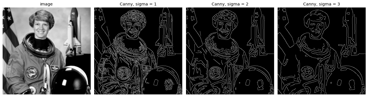
The single most important knob is the smoothing scale. A small \(\sigma\) keeps fine detail and texture, a large \(\sigma\) keeps only strong large-scale boundaries and gives cleaner but coarser contours. Choosing \(\sigma\) is choosing the scale of edges you care about.

astro = load_gray(data.astronaut())
fig, ax = plt.subplots(1, 4, figsize=(15, 4))
show(ax[0], astro, 'image')
for a, sig in zip(ax[1:], [1, 2, 3]):
    show(a, canny(astro, sigma=sig), f'Canny, sigma = {sig}')
plt.tight_layout(); plt.show()

.../site-packages/skimage/color/colorconv.py:984: RuntimeWarning: divide by zero encountered in matmul
  return rgb @ coeffs
.../site-packages/skimage/color/colorconv.py:984: RuntimeWarning: overflow encountered in matmul
  return rgb @ coeffs
.../site-packages/skimage/color/colorconv.py:984: RuntimeWarning: invalid value encountered in matmul
  return rgb @ coeffs

11. Beyond Canny: learned edge detection

Canny asks only whether intensity changes; it cannot tell a meaningful object boundary from busy texture or a soft shadow. Later work reframes edge detection as a learning problem trained on human-labelled boundaries. Martin et al. (2004) combine local brightness, colour, and texture cues into a learned pB boundary detector. Dollar and Zitnick (2013) train structured random forests to predict boundary patches quickly. Xie and Tu (2015) introduce Holistically-Nested Edge Detection (HED), a fully convolutional network with deep supervision that, by learning multi-scale features end to end, approaches human agreement on the BSDS500 benchmark and clearly outperforms Canny. The throughline is a shift from a fixed gradient rule to features and boundaries learned from data.

12. Explore and verify

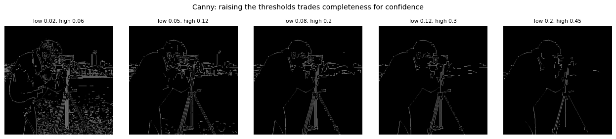
The derivative theorem of convolution is the claim that lets us smooth and differentiate in one pass. It is exactly checkable. So is the claim that non-maximum suppression only ever thins an edge map. We check both, then sweep Canny’s two thresholds.

# Verify the edge-detection claims.
import scipy.ndimage as ndi

im = load_gray(data.camera())

# 1. The derivative theorem of convolution. Convolution is associative, so
#    (im * g) * D  ==  im * (g * D): smoothing then differentiating is the same as
#    convolving once with a single combined kernel. That is what lets us do it in one pass.
#    gaussian_2d returns (xx, yy, g).
sigma, size = 2.0, 13
_, _, g = gaussian_2d(size, sigma)
D = np.array([[-0.5, 0.0, 0.5]])                       # central difference in x

two_passes = ndi.convolve(ndi.convolve(im, g, mode='reflect'), D, mode='reflect')
gD = ndi.convolve(np.pad(g, ((0, 0), (1, 1))), D, mode='constant')   # pad, or the kernel is clipped
one_pass = ndi.convolve(im, gD, mode='reflect')

m = (slice(20, -20), slice(20, -20))
assert np.allclose(two_passes[m], one_pass[m], atol=1e-12), 'derivative theorem fails'

# 2. Non-maximum suppression only ever thins: no new edge pixels, strictly fewer of them.
gx, gy = ndi.sobel(im, axis=1), ndi.sobel(im, axis=0)
mag, theta = np.hypot(gx, gy), np.arctan2(gy, gx)
thin = non_max_suppression(mag, theta)
assert np.all((thin > 0) <= (mag > 0)), 'NMS invented an edge pixel'
assert (thin > 0).sum() < (mag > 0).sum(), 'NMS did not thin anything'

print('both checks passed')
print(f'  two passes vs one combined {gD.shape[0]}x{gD.shape[1]} kernel: '
      f'max |difference| = {np.abs(two_passes[m] - one_pass[m]).max():.2e}')
print(f'  edge pixels before NMS: {(mag > 0).sum():6d}')
print(f'  edge pixels after  NMS: {(thin > 0).sum():6d}  ({100 * (thin > 0).sum() / (mag > 0).sum():.0f}% kept)')

both checks passed
  two passes vs one combined 13x15 kernel: max |difference| = 8.05e-16
  edge pixels before NMS: 255182
  edge pixels after  NMS:  90921  (36% kept)

# Static sweep: what the two hysteresis thresholds actually do.
# canny_edges returns (mag, thin, edges); we want the final edge map.
fig, ax = plt.subplots(1, 5, figsize=(15, 3.2))
for a, (lo, hi) in zip(ax, [(0.02, 0.06), (0.05, 0.12), (0.08, 0.20), (0.12, 0.30), (0.20, 0.45)]):
    edges = canny_edges(im, sigma=2, low=lo, high=hi)[2]
    a.imshow(edges, cmap='gray'); a.set_axis_off()
    a.set_title(f'low {lo}, high {hi}', fontsize=9)
fig.suptitle('Canny: raising the thresholds trades completeness for confidence', y=1.02)
plt.tight_layout(); plt.show()

Now the same thing under your control. Drag the slider and watch what changes.

# Live: all three Canny knobs at once.
from ipywidgets import interact, FloatSlider

def canny(sigma=2.0, low=0.08, high=0.20):
    if high <= low:
        high = low + 0.01
    edges = canny_edges(im, sigma=sigma, low=low, high=high)[2]
    fig, a = plt.subplots(figsize=(4.6, 4.6))
    a.imshow(edges, cmap='gray'); a.set_axis_off()
    a.set_title(f'$\sigma$={sigma:.1f}, low={low:.2f}, high={high:.2f}')
    plt.show()

interact(canny,
         sigma=FloatSlider(min=0.5, max=6, step=0.5, value=2.0),
         low=FloatSlider(min=0.01, max=0.30, step=0.01, value=0.08),
         high=FloatSlider(min=0.05, max=0.60, step=0.01, value=0.20));

---

Key takeaways

Concept	Key takeaway
Edges	Places of rapid intensity change; the derivative is large there
Finite differences	\(\partial f/\partial x\) is a correlation with \([-1, 0, 1]\)
Operators	Prewitt, Sobel, Roberts add smoothing along the edge; Sobel is the usual default
Gradient	\(\nabla f\) gives strength \(\lVert\nabla f\rVert\) and orientation \(\operatorname{atan2}(f_y, f_x)\)
Smoothing first	Differentiation amplifies noise, so low-pass before differentiating
Derivative of Gaussian	\(\frac{d}{dx}(f*g) = f * \frac{d}{dx}g\): smooth and differentiate in one kernel
Laplacian of Gaussian	Second-order operator; edges are zero-crossings, sharper but noisier
Non-max suppression	Keep local maxima along the gradient to get one-pixel ridges
Hysteresis	Two thresholds plus connectivity link strong and well-connected weak edges
Canny	DoG, then magnitude and orientation, then NMS, then hysteresis
\(\sigma\)	Sets edge scale: small keeps detail, large keeps coarse boundaries
Learned edges	pB, structured forests, and HED learn boundaries from labelled data

Reading: Szeliski, Computer Vision: Algorithms and Applications, Ch. 2 (and the edge-detection sections of Ch. 7 in the 2nd edition).

References: J. Canny (1986); D. Martin, C. Fowlkes, J. Malik (2004); P. Dollar, L. Zitnick (2013); P. Isola et al. (2014); S. Xie, Z. Tu (2015). Slide sources: K. Grauman, S. Seitz, R. Urtasun, D. Hoiem, N. Snavely, L. Lazebnik, J. Hays.

Exercises

1. One pass instead of two. Show that convolving with the derivative of a Gaussian equals smoothing then differentiating, using \(\frac{d}{dx}(f*g) = f * \frac{d}{dx}g\). Verify numerically and compare the cost.

2. What each Canny threshold does. Sweep the low and high hysteresis thresholds independently. Describe what raising each one removes, and find a setting that keeps a faint but real edge while dropping noise.

3. Operator robustness. Compare Prewitt, Sobel and Roberts on the same image with increasing noise. Which degrades first, and what does the smoothing built into Sobel buy you?

4. Zero-crossings versus Canny. Overlay LoG zero-crossings on Canny edges. Find a region where they disagree and explain which is closer to the true edge.