
📺 Lecture video | 📄 Slides
Week 3, Lecture 6: SGD and Adaptive Optimizers, Built From Scratch#
NPTEL Deep Learning for Computer Vision | Prof. Vineeth N Balasubramanian, IIT Hyderabad
Companion notebook for §3.3 Gradient Descent and Variants.
We start from batch gradient descent and work outward to the adaptive optimizers you use every day (Adagrad, RMSProp, Adam), coding every update rule by hand and watching it move on a loss surface.
What you will learn
The three update regimes: batch GD, stochastic GD (SGD), and mini-batch SGD, implemented from scratch, and why SGD is noisier but faster.
Learning rate schedules (step, exponential, 1/t decay) as plain functions of the iteration, plus one applied to training.
Adagrad, RMSProp, and Adam coded exactly as the slide equations, compared against plain SGD and momentum on a shared ill-conditioned surface.
A sanity check with
torch.optim.SGDandtorch.optim.Adamthat confirms the from-scratch intuition on a tiny network.
How we build it
From-scratch update rules first (plain numpy and torch tensors), so you see every
term, then the idiomatic torch.optim version at the end to confirm they agree.
How to run Colab CPU or GPU, or a local Jupyter. Every dataset is tiny and every cell finishes in a few seconds on CPU. Run the setup cell first.
Contents
Batch GD vs SGD vs Mini-batch SGD
Choosing the learning rate
Adaptive optimizers, coded from scratch
Sanity check with torch.optim
Review#
The previous lecture added momentum and Nesterov acceleration to plain gradient descent and watched them cross an ill-conditioned ravine. Both still use the whole dataset for every step. This lecture changes what each step sees, then makes the learning rate adapt per parameter.
Setup#
# Run this cell first. Works on Colab (CPU or GPU) and local Jupyter.
import sys, subprocess
# ipywidgets ships with Colab; install only if it is missing.
try:
    import ipywidgets  # noqa: F401
except ImportError:
    subprocess.run([sys.executable, "-m", "pip", "install", "-q", "ipywidgets"])

import numpy as np
import torch
import torch.nn as nn
import torch.nn.functional as F
import matplotlib.pyplot as plt
from ipywidgets import interact, interactive, FloatSlider, IntSlider, Dropdown, Checkbox, fixed
%matplotlib inline

# Reproducibility
torch.manual_seed(0)
np.random.seed(0)

# Use a GPU if one is available, otherwise CPU. Every demo here is tiny and
# runs in seconds on CPU, so no GPU is required.
device = torch.device("cuda" if torch.cuda.is_available() else "cpu")

plt.rcParams["figure.figsize"] = (7, 4.5)
plt.rcParams["axes.grid"] = True
plt.rcParams["axes.axisbelow"] = True

print("PyTorch", torch.__version__, "| device:", device)
PyTorch 2.8.0 | device: cpu
1. Batch GD vs SGD vs Mini-batch SGD#
All three minimize the same cost by stepping downhill, using the same update
They differ only in how much data each update uses.
Batch GD. Compute the gradient over the entire dataset, then take one step.
Pros: conditions of convergence are well understood; batch acceleration tricks (for example conjugate gradient) apply.
Cons: one step needs a full pass, which is painfully slow on large data. A single pass over ImageNet (about 14.2 million images) per update is a non-starter.
Stochastic GD (SGD). Shuffle the data and update after each example. Cheap and fast; the update noise can even help escape local minima and saddle points. The cost is a noisy path that may not settle without a good learning rate.
Mini-batch SGD. Update after a small batch of \(m\) examples (aggregate the gradient over the batch, then step). This is the default today and is usually just called “SGD”. Less noisy than \(m = 1\), still far more updates per pass than batch GD.
We fit a bias-free logistic regression (two weights \(w_1, w_2\), so the parameter path is 2D and easy to plot) on two Gaussian blobs, and run all three regimes from scratch: an inner loop over the full data, single examples, or mini-batches.
from sklearn.datasets import make_blobs

# Two Gaussian blobs, a tiny binary classification set. We center the features so
# a bias-free logistic model is enough, keeping the parameter vector 2D (w1, w2).
N = 300
Xnp, ynp = make_blobs(n_samples=N, centers=[[-2.0, -2.0], [2.0, 2.0]],
                      cluster_std=1.4, random_state=0)
Xnp = Xnp - Xnp.mean(axis=0, keepdims=True)
ynp = ynp.astype(np.float32)

X = torch.tensor(Xnp, dtype=torch.float32, device=device)
y = torch.tensor(ynp, dtype=torch.float32, device=device)

def full_loss(w):
    "Mean binary cross entropy over the whole dataset (no bias term)."
    with torch.no_grad():
        return F.binary_cross_entropy_with_logits(X @ w, y).item()

def train_regime(batch_size, lr=0.5, epochs=12, seed=0):
    "One from-scratch training run. batch_size = N is batch GD, 1 is SGD."
    g = torch.Generator().manual_seed(seed)
    w = torch.zeros(2, device=device, requires_grad=True)
    updates_per_epoch = int(np.ceil(N / batch_size))
    loss_hist, traj = [], []
    for _ in range(epochs):
        perm = torch.randperm(N, generator=g).to(device)   # shuffle each epoch
        for start in range(0, N, batch_size):
            idx = perm[start:start + batch_size]            # full data / 1 / m rows
            loss = F.binary_cross_entropy_with_logits(X[idx] @ w, y[idx])
            loss.backward()                                 # delta_theta = grad L
            with torch.no_grad():
                w -= lr * w.grad                            # theta <- theta - alpha*grad
                w.grad.zero_()
            loss_hist.append(full_loss(w))
            traj.append(w.detach().cpu().numpy().copy())
    # x-axis in epochs so all regimes are comparable per pass over the data.
    xs = np.arange(1, len(loss_hist) + 1) / updates_per_epoch
    return xs, np.array(loss_hist), np.array(traj)

print("dataset:", tuple(X.shape), "points, classes:", np.unique(ynp))
dataset: (300, 2) points, classes: [0. 1.]
# Loss surface over the two weights, used as the background for the trajectory.
gw = np.linspace(-1.0, 3.5, 70)
w1g, w2g = np.meshgrid(gw, gw)
logit_grid = w1g[..., None] * Xnp[:, 0] + w2g[..., None] * Xnp[:, 1]   # (70,70,N)
Z = np.mean(np.logaddexp(0.0, logit_grid) - ynp * logit_grid, axis=-1)  # mean BCE

# Same number of passes (epochs) over the data for a fair comparison.
xb, lb, tb = train_regime(N,  lr=0.5, epochs=12)   # Batch GD: 1 update per epoch
xs, ls, ts = train_regime(1,  lr=0.5, epochs=12)   # SGD: N updates per epoch
xm, lm, tm = train_regime(32, lr=0.5, epochs=12)   # Mini-batch: m = 32

fig, (axL, axR) = plt.subplots(1, 2, figsize=(12, 4.6))
axL.plot(xb, lb, color="#4c78a8", lw=2.2, label="Batch GD (m = N)")
axL.plot(xs, ls, color="#e45756", lw=0.7, alpha=0.85, label="SGD (m = 1)")
axL.plot(xm, lm, color="#54a24b", lw=1.3, label="Mini-batch (m = 32)")
axL.set_xlabel("epochs (full passes over the data)")
axL.set_ylabel("full-data BCE loss")
axL.set_title("Same 12 passes: SGD makes far more updates")
axL.legend()

axR.contourf(w1g, w2g, Z, levels=25, cmap="viridis", alpha=0.7)
axR.plot(tb[:, 0], tb[:, 1], "o-", color="#4c78a8", ms=4, lw=1.7, label="Batch GD")
axR.plot(ts[:, 0], ts[:, 1], ".-", color="#e45756", ms=2, lw=0.5, alpha=0.85, label="SGD")
axR.plot(tm[:, 0], tm[:, 1], ".-", color="#54a24b", ms=3, lw=1.0, label="Mini-batch")
axR.set_xlabel("w1")
axR.set_ylabel("w2")
axR.set_title("Parameter path (background: loss surface, dark = lower)")
axR.legend(loc="lower right")
plt.tight_layout()
plt.show()

print("final full-data loss:  batch %.4f   SGD %.4f   mini-batch %.4f" %
      (lb[-1], ls[-1], lm[-1]))
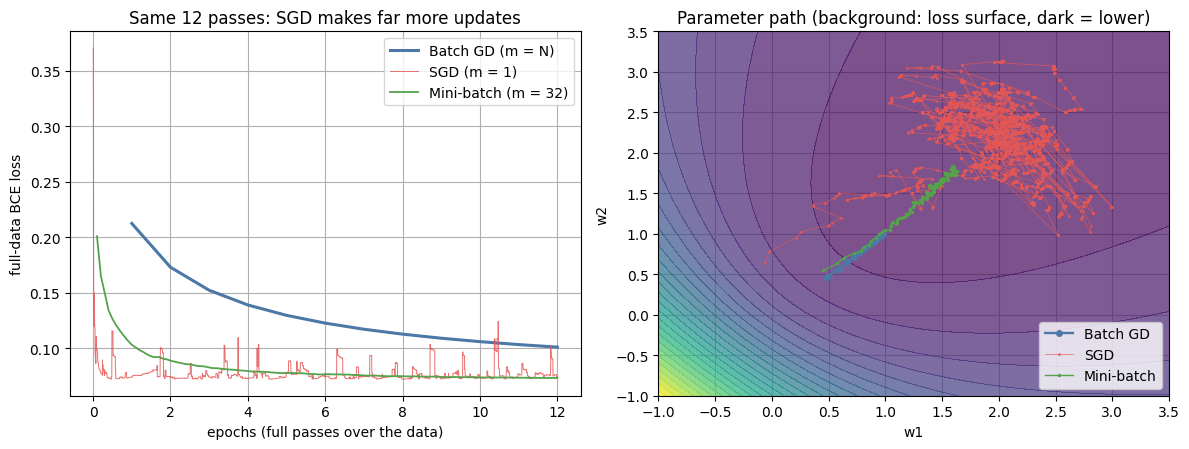
final full-data loss: batch 0.1011 SGD 0.0745 mini-batch 0.0734
Widget: batch size controls the noise#
Slide the batch size \(m\) from 1 (pure SGD, noisiest) up to \(N\) (full batch GD, smoothest). Watch the loss curve get noisier and the parameter path get more jagged as \(m\) shrinks, while small batches still make rapid progress because they take many updates per pass.
def batch_size_demo(batch_size=32):
    xs_, ls_, traj = train_regime(batch_size, lr=0.5, epochs=10)
    fig, (axL, axR) = plt.subplots(1, 2, figsize=(12, 4.6))
    axL.plot(xs_, ls_, color="#e45756", lw=0.9)
    axL.set_xlabel("epochs (full passes over the data)")
    axL.set_ylabel("full-data BCE loss")
    axL.set_title("Loss curve, batch size m = %d" % batch_size)
    axL.set_ylim(0.0, 0.75)
    axR.contourf(w1g, w2g, Z, levels=25, cmap="viridis", alpha=0.7)
    axR.plot(traj[:, 0], traj[:, 1], ".-", color="crimson", ms=3, lw=0.7)
    axR.set_xlabel("w1")
    axR.set_ylabel("w2")
    axR.set_title("Parameter path noise at m = %d (%d updates)" % (batch_size, len(traj)))
    plt.tight_layout()
    plt.show()

interact(batch_size_demo,
         batch_size=IntSlider(min=1, max=N, step=1, value=32));
2. Choosing the learning rate#
SGD lives or dies by its learning rate \(\alpha\). Too small and it crawls; too large and the gradients explode. A constant \(\alpha\) (naive linear search) is the simplest choice, but annealing \(\alpha\) over time usually helps: take large steps early, then small careful steps near the minimum.
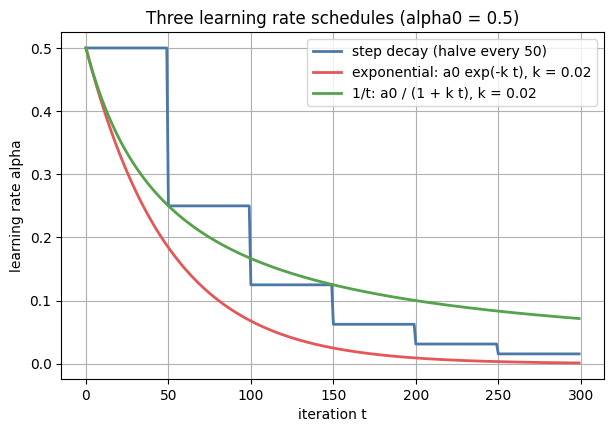
Three common schedules, as functions of the iteration \(t\):
Step decay: cut \(\alpha\) by a fixed factor every few iterations or epochs.
Exponential decay: \(\alpha = \alpha_0\, e^{-k t}\).
1/t decay: \(\displaystyle \alpha = \frac{\alpha_0}{1 + k t}\).
Here \(\alpha_0\) is the starting rate and \(k\) is a decay hyperparameter.
def step_decay(t, a0=0.5, drop=0.5, every=50):
    "Step decay: multiply the LR by 'drop' every 'every' iterations."
    return a0 * (drop ** np.floor(t / every))

def exp_decay(t, a0=0.5, k=0.02):
    "Exponential decay: alpha = alpha0 * exp(-k t)."
    return a0 * np.exp(-k * t)

def inv_t_decay(t, a0=0.5, k=0.02):
    "1/t decay: alpha = alpha0 / (1 + k t)."
    return a0 / (1.0 + k * t)

t = np.arange(0, 300)
plt.figure()
plt.plot(t, step_decay(t),            color="#4c78a8", lw=2, label="step decay (halve every 50)")
plt.plot(t, exp_decay(t, k=0.02),     color="#e45756", lw=2, label="exponential: a0 exp(-k t), k = 0.02")
plt.plot(t, inv_t_decay(t, k=0.02),   color="#54a24b", lw=2, label="1/t: a0 / (1 + k t), k = 0.02")
plt.xlabel("iteration t")
plt.ylabel("learning rate alpha")
plt.title("Three learning rate schedules (alpha0 = 0.5)")
plt.legend()
plt.show()
Widget: pick a schedule and its decay rate#
Choose the schedule and drag the decay rate \(k\) (which controls the exponential and 1/t curves; step decay uses its own fixed drop). Larger \(k\) means a faster decay.
def schedule_demo(schedule="exponential", k=0.02):
    t = np.arange(0, 300)
    if schedule == "step":
        a = step_decay(t)
    elif schedule == "exponential":
        a = exp_decay(t, k=k)
    else:
        a = inv_t_decay(t, k=k)
    plt.figure()
    plt.plot(t, a, color="#e45756", lw=2.2)
    plt.xlabel("iteration t")
    plt.ylabel("learning rate alpha")
    plt.title("%s schedule (k = %.3f, alpha0 = 0.5)" % (schedule, k))
    plt.ylim(0.0, 0.55)
    plt.show()

interact(schedule_demo,
         schedule=Dropdown(options=["step", "exponential", "1/t"], value="exponential"),
         k=FloatSlider(min=0.001, max=0.1, step=0.001, value=0.02));
One schedule applied to training#
A constant, largish learning rate keeps pure SGD bouncing around the minimum forever (the loss has a noisy floor). Decaying the same starting rate lets the steps shrink so the run settles into a lower, quieter loss. We print the standard deviation of the last 100 loss values to make the difference concrete.
def train_with_schedule(sched_fn, batch_size=1, epochs=6, seed=1):
    "Pure SGD (m = 1) where the learning rate at iteration t is sched_fn(t)."
    g = torch.Generator().manual_seed(seed)
    w = torch.zeros(2, device=device, requires_grad=True)
    losses, it = [], 0
    for _ in range(epochs):
        perm = torch.randperm(N, generator=g).to(device)
        for start in range(0, N, batch_size):
            idx = perm[start:start + batch_size]
            loss = F.binary_cross_entropy_with_logits(X[idx] @ w, y[idx])
            loss.backward()
            lr_t = float(sched_fn(it))
            with torch.no_grad():
                w -= lr_t * w.grad
                w.grad.zero_()
            losses.append(full_loss(w))
            it += 1
    return np.array(losses)

const_hist = train_with_schedule(lambda t: 1.5)
decay_hist = train_with_schedule(lambda t: exp_decay(t, a0=1.5, k=0.005))

plt.figure()
plt.plot(const_hist, color="#4c78a8", lw=0.8, alpha=0.9, label="constant alpha = 1.5")
plt.plot(decay_hist, color="#e45756", lw=1.3, label="exponential decay from 1.5")
plt.xlabel("SGD update iteration")
plt.ylabel("full-data BCE loss")
plt.title("A schedule applied to pure SGD: decay settles the noise")
plt.legend()
plt.show()

print("std of last 100 losses:  constant = %.4f   decayed = %.4f" %
      (const_hist[-100:].std(), decay_hist[-100:].std()))
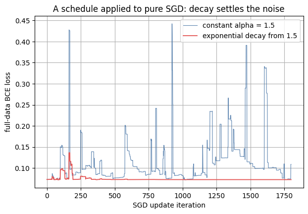
std of last 100 losses: constant = 0.0120 decayed = 0.0000
3. Adaptive optimizers, coded from scratch#
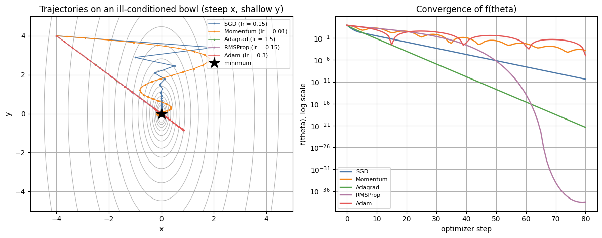
A single global learning rate is a blunt instrument: sparse or low-curvature directions want a bigger step than steep ones. Adaptive methods give each parameter its own effective learning rate, derived from the history of its gradients. We implement each update exactly as the slides state, with a small constant \(\delta\) for numeric stability.
Adagrad (accumulate squared gradients; steep directions get damped):
Per-parameter and adaptive, but \(r_t\) only grows, so the effective step decays toward zero and learning can stall.
RMSProp (fix Adagrad’s vanishing step with an exponentially decaying average):
Adam (combine momentum with RMSProp, plus bias correction):
The bias correction matters early, when \(s_t\) and \(r_t\) are still pulled toward their zero initial values. We also include plain momentum (\(v_t = \mu v_{t-1} + \Delta\theta_t\), then \(\theta_{t+1} = \theta_t - \alpha v_t\)) and plain SGD for comparison. The test surface is an ill-conditioned quadratic bowl, \(f(x, y) = \tfrac{1}{2}(10 x^2 + y^2)\): steep in \(x\), shallow in \(y\). Plain SGD zig-zags across the steep direction while crawling along the shallow one; the adaptive methods rescale per direction.
# An ill-conditioned quadratic bowl: curvature 10 in x, 1 in y (condition number 10).
Acurv = np.array([10.0, 1.0])

def f_surface(theta):
    "Loss f(theta) = 0.5 (10 x^2 + y^2)."
    return 0.5 * float(Acurv[0] * theta[0] ** 2 + Acurv[1] * theta[1] ** 2)

def grad_surface(theta):
    "Gradient of f: (10 x, y)."
    return Acurv * theta

def run_optimizer(name, lr, n_steps=80, start=(-4.0, 4.0),
                  mu=0.85, rho=0.9, rho1=0.9, rho2=0.999, delta=1e-8):
    "From-scratch optimizer, each branch matching the slide update equations."
    theta = np.array(start, dtype=np.float64)
    v = np.zeros(2); acc = np.zeros(2); r = np.zeros(2); s = np.zeros(2)
    traj = [theta.copy()]
    losses = [f_surface(theta)]
    for t in range(1, n_steps + 1):
        g = grad_surface(theta)                          # delta_theta_t = grad L
        if name == "SGD":
            theta = theta - lr * g
        elif name == "Momentum":
            v = mu * v + g
            theta = theta - lr * v
        elif name == "Adagrad":
            acc = acc + g ** 2                           # r_t = r_{t-1} + g^2
            theta = theta - lr / (delta + np.sqrt(acc)) * g
        elif name == "RMSProp":
            r = rho * r + (1 - rho) * g ** 2             # r_t = rho r + (1-rho) g^2
            theta = theta - lr / (delta + np.sqrt(r)) * g
        elif name == "Adam":
            s = rho1 * s + (1 - rho1) * g                # first moment
            r = rho2 * r + (1 - rho2) * g ** 2           # second moment
            s_hat = s / (1 - rho1 ** t)                  # bias correction
            r_hat = r / (1 - rho2 ** t)
            theta = theta - lr * s_hat / (delta + np.sqrt(r_hat))
        traj.append(theta.copy())
        losses.append(f_surface(theta))
    return np.array(traj), np.array(losses)

# Note: the slides use slightly different delta per method (about 1e-7 for Adagrad,
# 1e-6 for RMSProp, 1e-8 for Adam). One small delta is fine for this demo.
print("surface ready:  f(x, y) = 0.5 (10 x^2 + y^2), minimum at (0, 0)")
surface ready: f(x, y) = 0.5 (10 x^2 + y^2), minimum at (0, 0)
# Contour background for all section 3 plots.
gg = np.linspace(-5, 5, 120)
GX, GY = np.meshgrid(gg, gg)
GZ = 0.5 * (Acurv[0] * GX ** 2 + Acurv[1] * GY ** 2)
contour_levels = np.logspace(-1, 2.4, 18)

settings = [
    ("SGD",      0.15, "#4c78a8"),
    ("Momentum", 0.01, "#f58518"),
    ("Adagrad",  1.50, "#54a24b"),
    ("RMSProp",  0.15, "#b279a2"),
    ("Adam",     0.30, "#e45756"),
]

fig, (axT, axC) = plt.subplots(1, 2, figsize=(12, 4.8))
axT.contour(GX, GY, GZ, levels=contour_levels, colors="0.7", linewidths=0.8)
for name, lr, col in settings:
    traj, loss = run_optimizer(name, lr)
    axT.plot(traj[:, 0], traj[:, 1], ".-", color=col, ms=3, lw=1.1,
             label="%s (lr = %g)" % (name, lr))
    axC.plot(loss, color=col, lw=1.7, label=name)
axT.plot(0, 0, "k*", ms=16, label="minimum")
axT.set_xlim(-5, 5)
axT.set_ylim(-5, 5)
axT.set_xlabel("x")
axT.set_ylabel("y")
axT.set_title("Trajectories on an ill-conditioned bowl (steep x, shallow y)")
axT.legend(fontsize=8, loc="upper right")
axC.set_yscale("log")
axC.set_xlabel("optimizer step")
axC.set_ylabel("f(theta), log scale")
axC.set_title("Convergence of f(theta)")
axC.legend(fontsize=8)
plt.tight_layout()
plt.show()
Widget: optimizer and learning rate#
Pick an optimizer and a learning rate and watch its path on the bowl and its convergence curve. Things to try: push SGD’s learning rate up until it diverges; give Adagrad a large rate and watch it slow down on its own; see how Adam and RMSProp stay stable across a wide range.
def optimizer_demo(optimizer="Adam", lr=0.3):
    traj, loss = run_optimizer(optimizer, lr, n_steps=80)
    fig, (axT, axC) = plt.subplots(1, 2, figsize=(12, 4.8))
    axT.contour(GX, GY, GZ, levels=contour_levels, colors="0.7", linewidths=0.8)
    axT.plot(traj[:, 0], traj[:, 1], ".-", color="#e45756", ms=4, lw=1.2)
    axT.plot(0, 0, "k*", ms=16)
    axT.set_xlim(-5, 5)
    axT.set_ylim(-5, 5)
    axT.set_xlabel("x")
    axT.set_ylabel("y")
    axT.set_title("%s trajectory (lr = %.3f)" % (optimizer, lr))
    finite = np.isfinite(loss)
    axC.plot(np.arange(len(loss))[finite], np.clip(loss[finite], 1e-12, None),
             color="#e45756", lw=1.8)
    axC.set_yscale("log")
    axC.set_xlabel("optimizer step")
    axC.set_ylabel("f(theta), log scale")
    axC.set_title("Convergence (final f = %.2e)" % loss[-1])
    plt.tight_layout()
    plt.show()

interact(optimizer_demo,
         optimizer=Dropdown(options=["SGD", "Momentum", "Adagrad", "RMSProp", "Adam"], value="Adam"),
         lr=FloatSlider(min=0.005, max=1.5, step=0.005, value=0.3));
Widget: Adam’s momentum terms#
\(\beta_1\) (called \(\rho_1\) on the slide) controls the first-moment (momentum) average; \(\beta_2\) (\(\rho_2\)) controls the second-moment (RMSProp) average. The defaults 0.9 and 0.999 are the usual starting point. A lower \(\beta_2\) makes the per-parameter scaling react faster but noisier.
def adam_moments_demo(beta1=0.9, beta2=0.999):
    traj, loss = run_optimizer("Adam", lr=0.3, n_steps=80, rho1=beta1, rho2=beta2)
    fig, (axT, axC) = plt.subplots(1, 2, figsize=(12, 4.8))
    axT.contour(GX, GY, GZ, levels=contour_levels, colors="0.7", linewidths=0.8)
    axT.plot(traj[:, 0], traj[:, 1], ".-", color="#54a24b", ms=4, lw=1.2)
    axT.plot(0, 0, "k*", ms=16)
    axT.set_xlim(-5, 5)
    axT.set_ylim(-5, 5)
    axT.set_xlabel("x")
    axT.set_ylabel("y")
    axT.set_title("Adam with beta1 = %.3f, beta2 = %.4f" % (beta1, beta2))
    axC.plot(np.clip(loss, 1e-12, None), color="#54a24b", lw=1.8)
    axC.set_yscale("log")
    axC.set_xlabel("optimizer step")
    axC.set_ylabel("f(theta), log scale")
    axC.set_title("Convergence (final f = %.2e)" % loss[-1])
    plt.tight_layout()
    plt.show()

interact(adam_moments_demo,
         beta1=FloatSlider(min=0.5, max=0.99, step=0.01, value=0.9),
         beta2=FloatSlider(min=0.90, max=0.9999, step=0.0001, value=0.999));
4. Sanity check with torch.optim#
Everything above was hand-coded; in practice you call
torch.optim, which implements these exact update rules. We train one tiny
2-layer MLP on make_moons twice, once with torch.optim.SGD and once with
torch.optim.Adam, from the same initial weights, and compare the loss curves.
from sklearn.datasets import make_moons

Xmoon, ymoon = make_moons(n_samples=200, noise=0.2, random_state=0)
Xmoon = (Xmoon - Xmoon.mean(axis=0)) / Xmoon.std(axis=0)      # standardize
Xmoon_t = torch.tensor(Xmoon, dtype=torch.float32, device=device)
ymoon_t = torch.tensor(ymoon, dtype=torch.float32, device=device).unsqueeze(1)

def build_mlp(seed=0):
    "A tiny 2-16-1 MLP (same init every time we pass the same seed)."
    torch.manual_seed(seed)
    return nn.Sequential(nn.Linear(2, 16), nn.ReLU(), nn.Linear(16, 1)).to(device)

def train_with_optim(kind, lr, steps=150):
    "Full-batch training with a real torch.optim optimizer. Returns loss history."
    model = build_mlp(seed=0)
    if kind == "SGD":
        opt = torch.optim.SGD(model.parameters(), lr=lr)
    else:
        opt = torch.optim.Adam(model.parameters(), lr=lr)
    loss_fn = nn.BCEWithLogitsLoss()
    hist = []
    for _ in range(steps):
        opt.zero_grad()
        loss = loss_fn(model(Xmoon_t), ymoon_t)
        loss.backward()      # autograd computes the gradients
        opt.step()           # the optimizer applies exactly the rules from section 3
        hist.append(loss.item())
    return hist

hist_sgd = train_with_optim("SGD", lr=0.1)
hist_adam = train_with_optim("Adam", lr=0.05)

plt.figure()
plt.plot(hist_sgd,  color="#4c78a8", lw=1.8, label="torch.optim.SGD (lr = 0.1)")
plt.plot(hist_adam, color="#e45756", lw=1.8, label="torch.optim.Adam (lr = 0.05)")
plt.xlabel("training step")
plt.ylabel("BCE loss")
plt.title("torch.optim on a tiny 2-layer MLP (make_moons)")
plt.legend()
plt.show()

print("final loss:  SGD = %.4f   Adam = %.4f" % (hist_sgd[-1], hist_adam[-1]))
print("Adam's fast early descent matches the from-scratch intuition from section 3.")
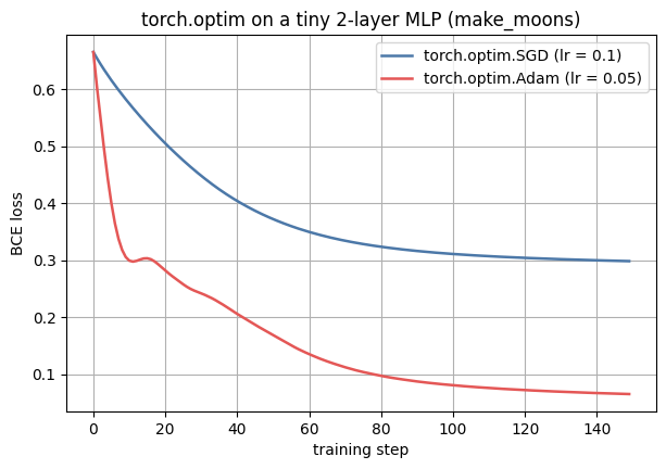
final loss:  SGD = 0.2983   Adam = 0.0651
Adam's fast early descent matches the from-scratch intuition from section 3.
Training neural nets with SGD: the challenges#
Real loss surfaces are non-convex, high-dimensional, and full of traps that make gradient descent hard:
Plateaus and flat regions where gradients are tiny.
Local minima and saddle points.
Vanishing and exploding gradients (and sharp cliffs).
Ill-conditioning (the steep versus shallow problem from section 3).
Inexact gradients and a poor match between local and global structure.
Choosing the learning rate and other hyperparameters.
There are no strong guarantees that training converges to a good solution, quickly, or at all. And yet, with the tools in this notebook, it works remarkably well in practice.
Key takeaways#
Batch GD, SGD, and mini-batch SGD use the same step \(\theta_{t+1} = \theta_t - \alpha\,\Delta\theta_t\); they differ only in how much data feeds each update. Mini-batch SGD (small \(m\)) is the practical default.
SGD’s noise is both a feature and a bug: it speeds things up and can escape saddles, but needs a sensible learning rate (often a decay schedule) to settle.
Schedules: step, exponential \(\alpha_0 e^{-k t}\), and 1/t \(\alpha_0 / (1 + k t)\).
Adaptive methods give each parameter its own step size from its gradient history: Adagrad accumulates \(g^2\) (and stalls), RMSProp decays that accumulator (no stall), and Adam adds momentum plus bias correction.
torch.optim.SGDandtorch.optim.Adamare exactly the from-scratch rules you coded here, just batteries included.
Exercises#
Answer the slide’s question: how could you tell whether you are stuck at a local minimum versus a saddle point on the loss surface? (Hint: think about the curvature, that is the eigenvalues of the Hessian.)
Change the surface in section 3 to a steeper condition number (say \(50 x^2 + y^2\)) and re-tune each optimizer. Which methods still work at the same learning rate?
Read DL Book Chapter 8 and the cs231n notes on SGD linked in the lecture.