Week 3, Lecture 9: Activation Functions In Depth

Week 3, Lecture 9: Activation Functions In Depth#

NPTEL Deep Learning for Computer Vision | Prof. Vineeth N Balasubramanian, IIT Hyderabad

Companion notebook for §3.5 Improvements in Training of Neural Networks.

We build the common activations from scratch, then use tiny PyTorch experiments to actually see why the choice of activation can make or break training.

What you will learn

The properties a good activation should have: continuous, differentiable, non-decreasing, cheap to compute.
Sigmoid, tanh, ReLU, Leaky ReLU, ELU coded from scratch (with their derivatives), verified against PyTorch.
Saturation: why sigmoid and tanh gradients collapse to almost $0$ away from the origin.
Vanishing gradients across depth (the central demo): per-layer gradient norms in a deep stack, sigmoid vs ReLU.
The Dying ReLU problem: how units go permanently silent, and how Leaky ReLU / ELU revive them.
The zero-centered issue: why all-positive activations force zig-zag weight updates.
A practical “which activation should I use” summary.

How to run Works on Colab (CPU or GPU) or a local Jupyter install. Every experiment here is tiny (single forward/backward passes on small tensors) and finishes in seconds on CPU. Run the setup cell below first, then go top to bottom.

Contents

The activation zoo, from scratch
Saturation, quantitatively
Vanishing gradients across depth (the central demo)
The Dying ReLU problem
The zero-centered issue (brief)

Review#

The previous lecture built early stopping, data augmentation, noise injection, ensembles and dropout, all of which control how a network fits its data. This lecture returns to a single component, the activation function, and shows how that choice alone can stop a deep network training at all.

Setup#

# Run this cell first. Works on Colab (CPU or GPU) and local Jupyter.
import sys, subprocess
# ipywidgets ships with Colab; install only if it is missing.
try:
    import ipywidgets  # noqa: F401
except ImportError:
    subprocess.run([sys.executable, "-m", "pip", "install", "-q", "ipywidgets"])

import numpy as np
import torch
import torch.nn as nn
import torch.nn.functional as F
import matplotlib.pyplot as plt
from ipywidgets import interact, interactive, FloatSlider, IntSlider, Dropdown, Checkbox, fixed
%matplotlib inline

# Reproducibility
torch.manual_seed(0)
np.random.seed(0)

# Use a GPU if one is available, otherwise CPU. Every demo here is tiny and
# runs in seconds on CPU, so no GPU is required.
device = torch.device("cuda" if torch.cuda.is_available() else "cpu")

plt.rcParams["figure.figsize"] = (7, 4.5)
plt.rcParams["axes.grid"] = True
plt.rcParams["axes.axisbelow"] = True

print("PyTorch", torch.__version__, "| device:", device)

PyTorch 2.8.0 | device: cpu

1. The activation zoo, from scratch#

An activation is a non-linear function applied to the output of a neuron. The slides ask what properties it should have. A good activation is:

continuous and differentiable (so we can backpropagate through it),
non-decreasing, and
easy to compute.

We work in three steps:

Implement each activation and its derivative directly from the math (no torch builtins).
Verify our from-scratch versions match PyTorch’s builtins and its autograd engine.
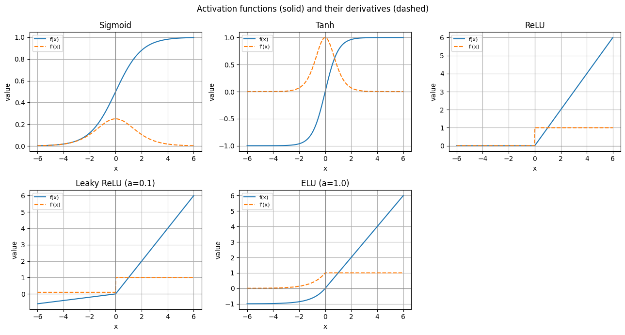
Plot every function next to its derivative.

Definitions from the slides:

Sigmoid: $\sigma(x) = \dfrac{1}{1+e^{-x}}$, with $\sigma'(x) = \sigma(x)\,\big(1-\sigma(x)\big)$. Squashes any input into $(0, 1)$.
Tanh: $\tanh(x) = \dfrac{e^{x}-e^{-x}}{e^{x}+e^{-x}}$, with $\tanh'(x) = 1-\tanh^2(x)$. Squashes into $(-1, 1)$.
ReLU: $\mathrm{ReLU}(x) = \max(0, x)$, with derivative $0$ for $x<0$ and $1$ for $x>0$.
Leaky ReLU: $\max(\alpha x,\, x)$, a small slope $\alpha$ for $x<0$.
ELU: $x$ for $x>0$, else $\alpha\,(e^{x}-1)$.

# Step 1: implement each activation and its analytic derivative directly from
# the slide math, using plain torch tensor ops (NOT the torch builtins).

def sigmoid(x):
    # sigma(x) = 1 / (1 + e^-x)
    return 1.0 / (1.0 + torch.exp(-x))

def d_sigmoid(x):
    # d sigma / dx = sigma(x) * (1 - sigma(x))
    s = sigmoid(x)
    return s * (1.0 - s)

def tanh(x):
    # tanh(x) = (e^x - e^-x) / (e^x + e^-x)
    ex, emx = torch.exp(x), torch.exp(-x)
    return (ex - emx) / (ex + emx)

def d_tanh(x):
    # d tanh / dx = 1 - tanh(x)^2
    t = tanh(x)
    return 1.0 - t * t

def relu(x):
    # ReLU(x) = max(0, x)
    return torch.clamp(x, min=0.0)

def d_relu(x):
    # derivative: 1 for x > 0, else 0 (we take 0 at the non-differentiable point)
    return (x > 0).to(x.dtype)

def leaky_relu(x, alpha=0.01):
    # Leaky ReLU keeps a small slope alpha for x < 0: max(alpha*x, x)
    return torch.where(x > 0, x, alpha * x)

def d_leaky_relu(x, alpha=0.01):
    # derivative: 1 for x > 0, else alpha
    return torch.where(x > 0, torch.ones_like(x), alpha * torch.ones_like(x))

def elu(x, alpha=1.0):
    # ELU(x) = x for x > 0, else alpha*(e^x - 1)
    return torch.where(x > 0, x, alpha * (torch.exp(x) - 1.0))

def d_elu(x, alpha=1.0):
    # derivative: 1 for x > 0, else alpha*e^x
    return torch.where(x > 0, torch.ones_like(x), alpha * torch.exp(x))

print("Defined from scratch: sigmoid, tanh, relu, leaky_relu, elu (and their derivatives).")

Defined from scratch: sigmoid, tanh, relu, leaky_relu, elu (and their derivatives).

# Step 2: verify our from-scratch versions agree with PyTorch. We check the
# FUNCTION values against torch builtins, and the DERIVATIVES against autograd
# (we let torch differentiate its own builtin and compare with our formula).
xv = torch.linspace(-6, 6, 200)

pairs = {
    "sigmoid": (sigmoid(xv),        torch.sigmoid(xv)),
    "tanh":    (tanh(xv),           torch.tanh(xv)),
    "relu":    (relu(xv),           torch.relu(xv)),
    "leaky":   (leaky_relu(xv, 0.1), F.leaky_relu(xv, 0.1)),
    "elu":     (elu(xv, 1.0),        F.elu(xv, 1.0)),
}
print("max |ours - torch| for the FUNCTION values:")
for name, (a, b) in pairs.items():
    print("  %-8s : %.2e" % (name, (a - b).abs().max().item()))

def autograd_deriv(fn, x):
    """Gradient of fn at each point via autograd (torch differentiates itself)."""
    x = x.clone().detach().requires_grad_(True)
    g, = torch.autograd.grad(fn(x).sum(), x)
    return g

print("\nmax |our derivative - autograd| for the DERIVATIVES:")
print("  sigmoid  : %.2e" % (d_sigmoid(xv) - autograd_deriv(torch.sigmoid, xv)).abs().max().item())
print("  tanh     : %.2e" % (d_tanh(xv)    - autograd_deriv(torch.tanh, xv)).abs().max().item())
print("  relu     : %.2e" % (d_relu(xv)    - autograd_deriv(torch.relu, xv)).abs().max().item())
print("  leaky    : %.2e" % (d_leaky_relu(xv, 0.1) - autograd_deriv(lambda t: F.leaky_relu(t, 0.1), xv)).abs().max().item())
print("  elu      : %.2e" % (d_elu(xv, 1.0) - autograd_deriv(lambda t: F.elu(t, 1.0), xv)).abs().max().item())

max |ours - torch| for the FUNCTION values:
  sigmoid  : 0.00e+00
  tanh     : 1.19e-07
  relu     : 0.00e+00
  leaky    : 0.00e+00
  elu      : 5.96e-08

max |our derivative - autograd| for the DERIVATIVES:
  sigmoid  : 0.00e+00
  tanh     : 2.38e-07
  relu     : 0.00e+00
  leaky    : 0.00e+00
  elu      : 0.00e+00

# Step 3: plot each activation (solid) next to its derivative (dashed).
grid = torch.linspace(-6, 6, 400)
gx = grid.numpy()
zoo = [
    ("Sigmoid",            sigmoid(grid),          d_sigmoid(grid)),
    ("Tanh",               tanh(grid),             d_tanh(grid)),
    ("ReLU",               relu(grid),             d_relu(grid)),
    ("Leaky ReLU (a=0.1)", leaky_relu(grid, 0.1),  d_leaky_relu(grid, 0.1)),
    ("ELU (a=1.0)",        elu(grid, 1.0),         d_elu(grid, 1.0)),
]
fig, axes = plt.subplots(2, 3, figsize=(13, 7))
for ax, (name, f, d) in zip(axes.ravel(), zoo):
    ax.plot(gx, f.numpy(), label="f(x)")
    ax.plot(gx, d.numpy(), "--", label="f'(x)")
    ax.axhline(0, color="gray", lw=0.8)
    ax.axvline(0, color="gray", lw=0.8)
    ax.set_title(name)
    ax.set_xlabel("x"); ax.set_ylabel("value")
    ax.legend(loc="upper left", fontsize=8)
axes.ravel()[-1].axis("off")   # 6th slot is unused
fig.suptitle("Activation functions (solid) and their derivatives (dashed)")
plt.tight_layout()
plt.show()

../../_images/c97ab40b13607793cb501a2e9127b220e3dea4fce6d60c0c7816437869eaa86a.png

Widget: explore each activation and its saturation region#

Pick an activation and move the parameter slider:

For sigmoid / tanh the slider is a gain $a$ (we plot $f(a\,x)$). A larger gain makes the curve steeper and pushes it into saturation sooner.
For Leaky ReLU the slider is the negative slope $\alpha$ (note $\alpha=0$ recovers plain ReLU).
For ELU the slider is $\alpha$.
ReLU has no parameter, so the slider is ignored.

The red band marks where $|f'(x)| < 0.1$: the saturation region, where the gradient is nearly zero and learning almost stops.

# WIDGET 1: dropdown activation + parameter slider -> redraw f and f' and shade
# the saturation region (|f'| < 0.1). All computation happens inside the callback.
def explore_activation(name="sigmoid", param=1.0):
    x = torch.linspace(-8, 8, 500)
    if name == "sigmoid":
        f, d, note = sigmoid(param * x), param * d_sigmoid(param * x), "gain a=%.2f" % param
    elif name == "tanh":
        f, d, note = tanh(param * x), param * d_tanh(param * x), "gain a=%.2f" % param
    elif name == "relu":
        f, d, note = relu(x), d_relu(x), "no parameter"
    elif name == "leaky_relu":
        f, d, note = leaky_relu(x, param), d_leaky_relu(x, param), "neg slope a=%.2f" % param
    else:  # elu
        f, d, note = elu(x, param), d_elu(x, param), "alpha=%.2f" % param
    gx = x.numpy(); fn = f.numpy(); dn = d.numpy()
    sat = np.abs(dn) < 0.1

    plt.figure()
    plt.plot(gx, fn, label="f(x)")
    plt.plot(gx, dn, "--", label="f'(x)")
    plt.axhline(0, color="gray", lw=0.8); plt.axvline(0, color="gray", lw=0.8)
    y0, y1 = plt.ylim()
    plt.fill_between(gx, y0, y1, where=sat, color="red", alpha=0.15,
                     label="saturation |f'| < 0.1")
    plt.ylim(y0, y1)
    plt.title("%s (%s): function, derivative, saturation region" % (name, note))
    plt.xlabel("x"); plt.ylabel("value"); plt.legend(loc="upper left", fontsize=8)
    plt.show()

interact(explore_activation,
         name=Dropdown(options=["sigmoid", "tanh", "relu", "leaky_relu", "elu"], value="sigmoid"),
         param=FloatSlider(min=0.0, max=3.0, step=0.05, value=1.0));

2. Saturation, quantitatively#

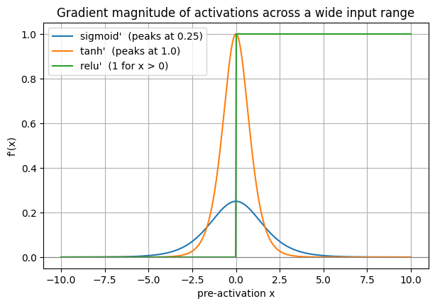
“Saturation” means the function flattens out, so its derivative goes to (almost) zero. Since a weight update is proportional to the gradient, a saturated neuron barely learns: the slide notes that the gradient of a sigmoid neuron at saturation is very small, which makes training slow.

Sigmoid’s derivative peaks at only $0.25$ (at $x=0$) and decays to $\approx 0$ for $|x| \gtrsim 5$.
Tanh’s derivative peaks at $1.0$ (at $x=0$) but also decays to $\approx 0$ in the tails.
ReLU’s derivative is a flat $1$ for every positive input: no saturation on the positive side.

# Plot the gradient magnitude of each activation across a wide input range.
x = torch.linspace(-10, 10, 600)
gx = x.numpy()
plt.figure()
plt.plot(gx, d_sigmoid(x).numpy(), label="sigmoid'  (peaks at 0.25)")
plt.plot(gx, d_tanh(x).numpy(),    label="tanh'  (peaks at 1.0)")
plt.plot(gx, d_relu(x).numpy(),    label="relu'  (1 for x > 0)")
plt.axhline(0, color="gray", lw=0.8)
plt.title("Gradient magnitude of activations across a wide input range")
plt.xlabel("pre-activation x"); plt.ylabel("f'(x)")
plt.legend()
plt.show()

# How fast does the sigmoid gradient collapse away from 0?
print("How the derivative shrinks as we move away from the origin:")
for x0 in [0, 1, 3, 5, 8]:
    t = torch.tensor([float(x0)])
    print("  |x|=%d :  sigmoid'=%.4f   tanh'=%.4f   relu'=%.0f" %
          (x0, d_sigmoid(t).item(), d_tanh(t).item(), d_relu(t).item()))

../../_images/f0515537d7a426668f4ab47940f6f25a1b407e6a81faff94a3566ebb7aea3ba6.png

How the derivative shrinks as we move away from the origin:
  |x|=0 :  sigmoid'=0.2500   tanh'=1.0000   relu'=0
  |x|=1 :  sigmoid'=0.1966   tanh'=0.4200   relu'=1
  |x|=3 :  sigmoid'=0.0452   tanh'=0.0099   relu'=1
  |x|=5 :  sigmoid'=0.0066   tanh'=0.0002   relu'=1
  |x|=8 :  sigmoid'=0.0003   tanh'=0.0000   relu'=1

Widget: read the gradient at any input#

Slide the input point $x_0$. The title reports each activation’s gradient there. Notice that by $|x_0| = 5$ the sigmoid and tanh gradients are essentially zero (learning stalls), while ReLU stays at exactly $1$ for any positive input. Small gradient means a tiny weight update means slow learning.

# WIDGET 2: slide the input point x0 and read each activation's gradient there.
def gradient_at(x0=4.0):
    x = torch.linspace(-10, 10, 600); gx = x.numpy()
    xt = torch.tensor([float(x0)])
    ds, dt, dr = d_sigmoid(xt).item(), d_tanh(xt).item(), d_relu(xt).item()
    plt.figure()
    plt.plot(gx, d_sigmoid(x).numpy(), label="sigmoid'")
    plt.plot(gx, d_tanh(x).numpy(),    label="tanh'")
    plt.plot(gx, d_relu(x).numpy(),    label="relu'")
    plt.axvline(x0, color="k", ls=":")
    plt.scatter([x0, x0, x0], [ds, dt, dr], color="black", zorder=5)
    plt.title("Gradient at x=%.1f:  sigmoid=%.4f, tanh=%.4f, relu=%.0f" % (x0, ds, dt, dr))
    plt.xlabel("pre-activation x"); plt.ylabel("f'(x)"); plt.legend()
    plt.show()

interact(gradient_at, x0=FloatSlider(min=-10.0, max=10.0, step=0.5, value=4.0));

3. Vanishing gradients across depth (the central demo)#

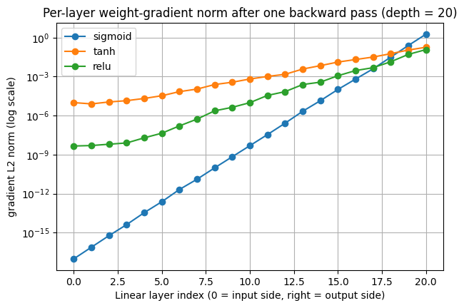
Backprop multiplies gradients layer by layer. Each saturating activation contributes a factor of at most $0.25$ (sigmoid) or $1$ (tanh), so after many layers the product shrinks toward zero by the time it reaches the early layers. Those layers then receive almost no gradient and learn painfully slowly. This is the vanishing gradient problem, and it is the main reason plain sigmoid/tanh stacks are hard to train when deep.

We stack depth blocks of Linear + activation, run a single backward pass from a random loss, and read the gradient L2-norm of each layer’s weights. Watch how the sigmoid and tanh norms fall off toward the input side (left bars), while ReLU keeps them far healthier.

# Build a deep stack of Linear + activation, do ONE backward pass, and collect
# the gradient L2-norm of each Linear layer's weight. Tiny and fast on CPU.
def build_deep_net(depth, width=32, act="sigmoid"):
    acts = {"sigmoid": nn.Sigmoid, "tanh": nn.Tanh, "relu": nn.ReLU}
    layers = []
    for _ in range(depth):
        layers.append(nn.Linear(width, width))
        layers.append(acts[act]())
    layers.append(nn.Linear(width, 1))       # scalar-ish head so we get one loss
    return nn.Sequential(*layers).to(device)

def per_layer_grad_norms(depth=20, act="sigmoid", width=32, batch=64):
    torch.manual_seed(0)                      # same init and data across activations
    net = build_deep_net(depth, width, act)
    x = torch.randn(batch, width, device=device)
    target = torch.randn(batch, 1, device=device)
    loss = F.mse_loss(net(x), target)
    net.zero_grad()
    loss.backward()
    return [m.weight.grad.norm().item() for m in net if isinstance(m, nn.Linear)]

# Static comparison at a fixed depth: sigmoid vs tanh vs relu.
depth0 = 20
plt.figure()
for act in ["sigmoid", "tanh", "relu"]:
    norms = per_layer_grad_norms(depth0, act)
    plt.plot(range(len(norms)), np.maximum(norms, 1e-30), marker="o", label=act)
plt.yscale("log")
plt.title("Per-layer weight-gradient norm after one backward pass (depth = %d)" % depth0)
plt.xlabel("Linear layer index (0 = input side, right = output side)")
plt.ylabel("gradient L2 norm (log scale)")
plt.legend()
plt.show()

../../_images/e33fa398ac0fad808246eef78703afde1d1c2e5c409a8a635a8d29f373660ecd.png

Widget: depth vs activation#

Increase the depth and switch the activation. With sigmoid (and, less severely, tanh) the left-most bars (near the input) drop by many orders of magnitude as depth grows: that is the vanishing gradient. ReLU’s non-saturating positive region keeps the gradient far healthier all the way to the input side.

# WIDGET 3: depth slider + activation dropdown -> per-layer gradient bar chart.
def vanishing_demo(depth=15, act="sigmoid"):
    norms = per_layer_grad_norms(depth, act)
    plt.figure()
    plt.bar(range(len(norms)), np.maximum(norms, 1e-30), color="steelblue")
    plt.yscale("log")
    plt.title("Vanishing-gradient check: %s, depth = %d" % (act, depth))
    plt.xlabel("Linear layer index (0 = input side)")
    plt.ylabel("gradient L2 norm (log scale)")
    plt.show()

interact(vanishing_demo,
         depth=IntSlider(min=5, max=30, step=1, value=15),
         act=Dropdown(options=["sigmoid", "tanh", "relu"], value="sigmoid"));

4. The Dying ReLU problem#

ReLU’s gradient is exactly $0$ for $x<0$. If a unit’s pre-activation is negative for every input in the batch, then its output is always $0$ and its gradient is always $0$, so its incoming weights never update. It becomes a permanently “dead” neuron. A strongly negative bias (which a too-large learning-rate step can produce) pushes many units into exactly this state.

Fixes from the slides:

Initialize the bias to a small positive value.
Use Leaky ReLU $\max(\alpha x, x)$ or ELU: both keep a non-zero slope for $x<0$, so a non-firing unit still receives a gradient and can recover.

We take a layer of units, push their biases negative, and count the dead-unit fraction (units whose pre-activation is negative for the whole batch). Then we switch on a Leaky slope and watch that fraction fall.

# A unit is "dead" (for ReLU) if its pre-activation is <= 0 for the WHOLE batch.
# With a Leaky/ELU slope alpha > 0, even a non-firing unit has gradient alpha != 0,
# so it is never truly dead.
def dead_stats(neg_bias=3.0, alpha=0.0, n_units=300, d_in=20, n_samples=256):
    torch.manual_seed(0)
    W = torch.randn(n_units, d_in, device=device) / (d_in ** 0.5)   # ~unit-variance pre-acts
    b = -neg_bias + 0.5 * torch.randn(n_units, device=device)       # push biases negative
    X = torch.randn(n_samples, d_in, device=device)
    pre = X @ W.t() + b                        # (n_samples, n_units) pre-activations
    fire_rate = (pre > 0).float().mean(dim=0)  # fraction of the batch each unit fires on
    dead_relu = (fire_rate == 0).float().mean().item()
    dead_effective = dead_relu if alpha == 0 else 0.0
    return fire_rate.cpu().numpy(), dead_relu, dead_effective

fr, dead_relu, _ = dead_stats(neg_bias=3.0, alpha=0.0)
print("Negative bias offset 3.0, plain ReLU:")
print("  dead-unit fraction = %.1f%%  (these units never fire, so their gradient is always 0)" %
      (100 * dead_relu))
_, _, dead_leaky = dead_stats(neg_bias=3.0, alpha=0.1)
print("Same layer with Leaky ReLU (alpha=0.1):")
print("  dead-unit fraction = %.1f%%  (non-zero negative slope revives every unit)" %
      (100 * dead_leaky))

Negative bias offset 3.0, plain ReLU:
  dead-unit fraction = 58.0%  (these units never fire, so their gradient is always 0)
Same layer with Leaky ReLU (alpha=0.1):
  dead-unit fraction = 0.0%  (non-zero negative slope revives every unit)

Widget: kill units, then revive them#

Raise neg_bias to push more units below zero for the whole batch: the left histogram piles up at a firing rate of $0$ and the dead-unit fraction climbs. Now raise the Leaky slope alpha above $0$: because the negative side then has slope $\alpha \neq 0$, no unit has a zero gradient anymore, so the dead fraction drops to $0$ (the units can learn their way back). ELU behaves the same way, since its negative-side derivative $\alpha e^{x}$ is also non-zero.

# WIDGET 4: neg_bias slider (kills units) + Leaky alpha slider (revives them).
def dying_relu_demo(neg_bias=3.0, alpha=0.0):
    fr, dead_relu, dead_eff = dead_stats(neg_bias, alpha)
    fig, (ax1, ax2) = plt.subplots(1, 2, figsize=(12, 4.2))
    ax1.hist(fr, bins=20, range=(0, 1), color="steelblue")
    ax1.set_title("Per-unit firing rate (plain ReLU dead = %.1f%%)" % (100 * dead_relu))
    ax1.set_xlabel("fraction of batch that activates the unit")
    ax1.set_ylabel("number of units")
    ax2.bar(["plain ReLU", "Leaky (a=%.2f)" % alpha], [dead_relu, dead_eff],
            color=["salmon", "seagreen"])
    ax2.set_ylim(0, 1)
    ax2.set_ylabel("fraction of units with zero gradient (dead)")
    ax2.set_title("Dead units: ReLU vs Leaky / ELU")
    plt.tight_layout()
    plt.show()

interact(dying_relu_demo,
         neg_bias=FloatSlider(min=0.0, max=6.0, step=0.25, value=3.0),
         alpha=FloatSlider(min=0.0, max=0.3, step=0.01, value=0.0));

5. The zero-centered issue (brief)#

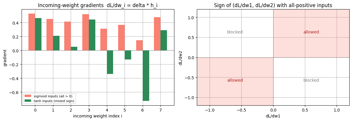
From the slides, for a neuron whose pre-activation is $a = \sum_i w_i h_i$ feeding an output $y$, the gradient of each incoming weight is $$\frac{\partial L}{\partial w_i} = \frac{\partial L}{\partial y}\,\frac{\partial y}{\partial a}\,h_i = \delta\, h_i,$$ where the factor $\delta = \frac{\partial L}{\partial y}\frac{\partial y}{\partial a}$ is **shared** by all incoming weights. If the inputs $h_i$ are sigmoid outputs they are **all positive**, so every $\partial L/\partial w_i$ takes the sign of $\delta$: all incoming weights want to move the same way at once. With only “all up” or “all down” moves available, the update path has to zig-zag toward the optimum. Tanh outputs are zero-centered (mixed signs), which unblocks the other update directions.

The plot below shows the incoming-weight gradients for one neuron (left), and the directions the weight vector is allowed to move in the 2-weight case (right).

# All-positive (sigmoid) inputs force every incoming-weight gradient to share the
# sign of the shared upstream factor delta. Tanh inputs are zero-centered (mixed).
torch.manual_seed(1)
delta = 0.8                          # a single shared upstream scalar for this neuron
z = torch.randn(8)                   # raw pre-activations from the previous layer
h_sig = sigmoid(z)                   # all positive  -> not zero-centered
h_tanh = tanh(z)                     # mixed sign     -> zero-centered
g_sig = (delta * h_sig).numpy()      # incoming-weight gradients with sigmoid inputs
g_tanh = (delta * h_tanh).numpy()    # incoming-weight gradients with tanh inputs

fig, (ax1, ax2) = plt.subplots(1, 2, figsize=(12, 4.2))
idx = np.arange(8)
ax1.bar(idx - 0.18, g_sig, width=0.36, label="sigmoid inputs (all > 0)", color="salmon")
ax1.bar(idx + 0.18, g_tanh, width=0.36, label="tanh inputs (mixed sign)", color="seagreen")
ax1.axhline(0, color="gray", lw=0.8)
ax1.set_title("Incoming-weight gradients  dL/dw_i = delta * h_i")
ax1.set_xlabel("incoming weight index i"); ax1.set_ylabel("gradient")
ax1.legend(fontsize=8)

# 2-weight picture: with h1, h2 > 0 the gradient (delta*h1, delta*h2) can only sit
# in quadrant I (both +) or III (both -). Shade those "allowed" quadrants.
ax2.axhline(0, color="gray", lw=0.8); ax2.axvline(0, color="gray", lw=0.8)
ax2.fill_between([0, 1.2], 0, 1.2, color="salmon", alpha=0.25)
ax2.fill_between([-1.2, 0], -1.2, 0, color="salmon", alpha=0.25)
ax2.text(0.6, 0.6, "allowed", ha="center", color="firebrick")
ax2.text(-0.6, -0.6, "allowed", ha="center", color="firebrick")
ax2.text(-0.6, 0.6, "blocked", ha="center", color="gray")
ax2.text(0.6, -0.6, "blocked", ha="center", color="gray")
ax2.set_xlim(-1.2, 1.2); ax2.set_ylim(-1.2, 1.2)
ax2.set_title("Sign of (dL/dw1, dL/dw2) with all-positive inputs")
ax2.set_xlabel("dL/dw1"); ax2.set_ylabel("dL/dw2")
plt.tight_layout()
plt.show()

print("sigmoid-input gradient signs:", np.sign(g_sig).astype(int), " (all the same)")
print("tanh-input gradient signs:   ", np.sign(g_tanh).astype(int), " (mixed)")

../../_images/ca180f1af0bd4159ba9e30d974f374771958b5cf51886abdff54d332c52694b1.png

sigmoid-input gradient signs: [1 1 1 1 1 1 1 1]  (all the same)
tanh-input gradient signs:    [ 1  1  1  1 -1 -1 -1  1]  (mixed)

Key takeaways and which activation to choose#

Good activations are continuous, differentiable, non-decreasing, and cheap.
Sigmoid: saturates (tiny gradients far from $0$), is not zero-centered (zig-zag updates), and uses an expensive exp. Rarely used in vanilla nets today; mainly kept for gating.
Tanh: zero-centered (better than sigmoid), but still saturates and still uses exp.
ReLU: non-saturating for positive inputs, converges much faster (about 6x in AlexNet), and is cheap. The default choice today, but watch for dead units.
Leaky ReLU / ELU / Maxout: variants that avoid dead units by keeping a non-zero negative-side slope.

Practical recipe (straight from the slides):

Use ReLU by default; be careful with learning rates and monitor the fraction of dead units.
Try Leaky ReLU, ELU, Maxout.
Try tanh, but expect worse performance.
Use sigmoid only when a gating is required.
In general it is good for an activation to stay in its (near) linear region for most of training.

Exercises#

in section 3, switch the deep net to tanh and compare its per-layer gradient decay against sigmoid and relu. Then, in section 4, replace the negative bias with a small positive bias and confirm the dead-unit fraction drops toward $0$. Bonus: add GELU or Maxout to the section 1 zoo, implemented from scratch, and verify it against PyTorch.