
📺 Lecture video | 📄 Slides
Week 2, Lecture 5: Image Segmentation#
NPTEL Deep Learning for Computer Vision | Prof. Vineeth N Balasubramanian, IIT Hyderabad
Companion notebook for §2.5 Image Segmentation.
What you will learn
Frame segmentation as a grouping problem, guided by Gestalt cues.
Apply watershed segmentation, and superpixels with region merging.
Use graph-based segmentation and probabilistic aggregation.
Apply mean shift and normalized cuts, and see where each one fails.
Contents
Segmentation and Gestalt grouping
Watershed segmentation
Superpixels and region merging
Graph-based segmentation
Probabilistic aggregation
Mean shift
Normalized cuts
Other methods and beyond images
How to run Runs on Colab or a local Jupyter, CPU only. Needs opencv-python alongside scikit-image and scipy; Colab ships all three. Run the setup cell first, then go top to bottom.
Review#
The previous lectures built local features: detectors and descriptors that pick out and describe individual keypoints. Segmentation asks the complementary question: how do we group pixels into coherent regions?
Image segmentation partitions an image into regions whose pixels belong together, by color, texture, or spatial continuity. It is one of the oldest problems in vision, and the classical methods below (watershed, superpixels, graph cuts, mean shift, normalized cuts) still appear as building blocks and preprocessing steps inside modern deep pipelines. This lecture walks through the main families and shows each one running on a real image.
Setup#
Everything runs offline on images bundled with scikit-image, plus a few synthetic patterns. We use scikit-image for watershed, SLIC and Felzenszwalb segmentation, OpenCV for k-means and mean-shift filtering, and plain NumPy or SciPy for the from-scratch demos.
%matplotlib inline
import numpy as np
import matplotlib.pyplot as plt
from scipy import ndimage as ndi
from skimage import data, util, color
import cv2

np.random.seed(0)
plt.rcParams['figure.figsize'] = (10, 4)
plt.rcParams['image.cmap']     = 'gray'
plt.rcParams['figure.dpi']     = 85

def show(ax, im, title='', cmap=None):
    ax.imshow(im, cmap=cmap); ax.set_title(title); ax.axis('off')

def to_u8(im):                                  # float image in [0,1] to uint8 for OpenCV
    return (np.clip(im, 0, 1) * 255).astype(np.uint8)
1. Segmentation and Gestalt grouping#
Long before algorithms, Gestalt psychology (early 20th century) described how human vision groups parts into wholes. Its slogan, the whole is greater than the sum of its parts, captures the idea that we perceive organized groups rather than isolated dots and edges.
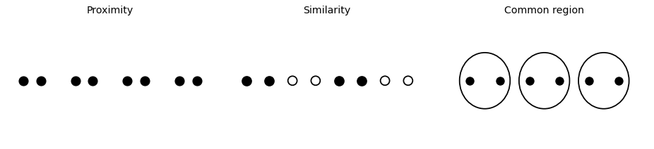
Gestalt theory lists cues that make elements group together:
Proximity: nearby elements are seen as one group.
Similarity: elements that look alike group together.
Common region, closure, continuity, parallelism, symmetry, common fate: enclosure, completion, smooth continuation, and shared motion all bind elements.
These rules are descriptive, not algorithmic: they explain why a grouping looks right, but they are too loose to directly produce a segmentation. The methods that follow turn these intuitions into computable criteria.
from matplotlib.patches import Ellipse

fig, axes = plt.subplots(1, 3, figsize=(11, 2.6))

# Proximity: dots fall into perceptual pairs by spacing alone
ax = axes[0]
xs = np.array([0, 1, 3, 4, 6, 7, 9, 10], float)
ax.scatter(xs, np.zeros_like(xs), s=120, c='k')
ax.set_title('Proximity'); ax.set_xlim(-1, 11); ax.set_ylim(-1, 1); ax.axis('off')

# Similarity: filled vs open circles group by appearance
ax = axes[1]
fills = ['k', 'k', 'none', 'none', 'k', 'k', 'none', 'none']
for x, f in zip(range(8), fills):
    ax.scatter([x], [0], s=120, facecolors=f, edgecolors='k', linewidths=1.5)
ax.set_title('Similarity'); ax.set_xlim(-1, 8); ax.set_ylim(-1, 1); ax.axis('off')

# Common region: enclosure overrides equal spacing
ax = axes[2]
ax.scatter(range(6), np.zeros(6), s=90, c='k')
for cx in [0.5, 2.5, 4.5]:
    ax.add_patch(Ellipse((cx, 0), 1.7, 0.9, fill=False, lw=1.5))
ax.set_title('Common region'); ax.set_xlim(-1, 6); ax.set_ylim(-1, 1); ax.axis('off')

plt.tight_layout(); plt.show()
2. Watershed segmentation#
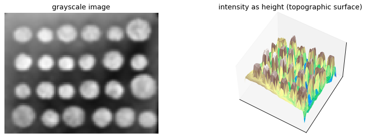
The watershed method (Beucher and Lantuejoul, 1979) reads a grayscale image as a topographic surface: intensity is height, so bright pixels are peaks and dark pixels are valleys. If we flood the surface from local minima, water from different minima fills separate catchment basins, and the ridges where two floods meet become watershed lines, the region boundaries.
A few practical points:
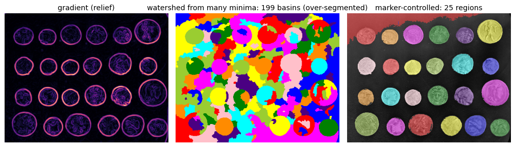
Watershed is usually run on the gradient magnitude, not the raw image, so that basins fall on smooth regions and ridges sit on strong edges.
Flooding from every local minimum over-segments: noise creates many spurious minima, hence many tiny regions.
The fix is marker-controlled watershed: place one marker inside each object (often from a distance transform) and flood only from those markers.
img = util.img_as_float(data.coins())
small = ndi.gaussian_filter(ndi.zoom(img, 0.25, order=1), 1.0)   # downsample for a readable surface
yy, xx = np.mgrid[0:small.shape[0], 0:small.shape[1]]

fig = plt.figure(figsize=(11, 3.4))
ax1 = fig.add_subplot(1, 2, 1)
ax1.imshow(small, cmap='gray'); ax1.set_title('grayscale image'); ax1.axis('off')

ax2 = fig.add_subplot(1, 2, 2, projection='3d')
ax2.plot_surface(xx, yy, small, cmap='terrain', linewidth=0, antialiased=True)
ax2.set_title('intensity as height (topographic surface)')
ax2.set_xticks([]); ax2.set_yticks([]); ax2.set_zticks([]); ax2.view_init(elev=55, azim=-60)
plt.tight_layout(); plt.show()
from skimage.filters import sobel, threshold_otsu
from skimage.feature import peak_local_max
from skimage.segmentation import watershed

coins = util.img_as_float(data.coins())
grad  = sobel(ndi.gaussian_filter(coins, 1.0))

# Naive: seed a basin at every local minimum of the gradient -> far too many regions
seeds = peak_local_max(grad.max() - grad, min_distance=10)
m = np.zeros(grad.shape, bool); m[tuple(seeds.T)] = True
markers_over, _ = ndi.label(m)
ws_over = watershed(grad, markers_over)

# Marker-controlled: one marker per coin from the distance transform inside the foreground
bw   = ndi.binary_fill_holes(coins > threshold_otsu(coins))
dist = ndi.distance_transform_edt(bw)
peaks = peak_local_max(dist, min_distance=20, labels=bw)
mm = np.zeros(dist.shape, bool); mm[tuple(peaks.T)] = True
markers, _ = ndi.label(mm)
ws_marked = watershed(-dist, markers, mask=bw)

fig, ax = plt.subplots(1, 3, figsize=(12, 3.3))
show(ax[0], grad, 'gradient (relief)', cmap='magma')
show(ax[1], color.label2rgb(ws_over, bg_label=0),
     f'watershed from many minima: {ws_over.max()} basins (over-segmented)')
show(ax[2], color.label2rgb(ws_marked, image=coins, bg_label=0, alpha=0.4),
     f'marker-controlled: {ws_marked.max()} regions')
plt.tight_layout(); plt.show()
3. Superpixels and region merging#
Two broad strategies build regions incrementally:
Region splitting starts from the whole image and cuts it into finer pieces.
Region merging starts from pixels and repeatedly merges similar neighbors.
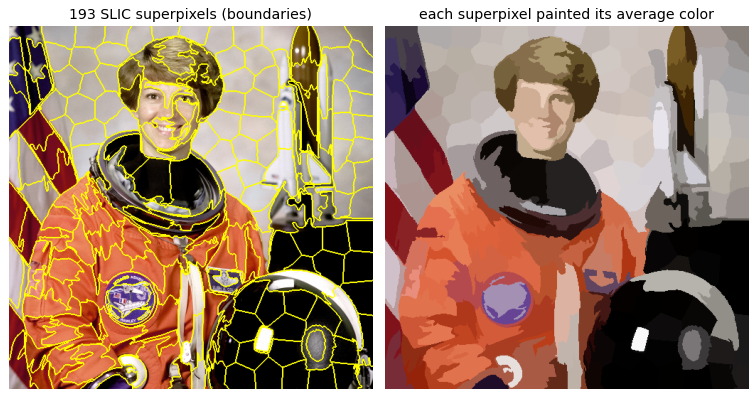
A popular merging result is the superpixel: a small, compact group of pixels of near-uniform color. SLIC (Achanta et al., 2012) produces them by running a localized k-means in a combined color-and-position space. Superpixels are rarely the final answer; they are a compact preprocessing layer, replacing a million pixels with a few hundred regions that higher-level algorithms then group further.
from skimage.segmentation import slic, mark_boundaries

img = util.img_as_float(data.astronaut())
seg = slic(img, n_segments=250, compactness=10, sigma=1, start_label=1)
avg = color.label2rgb(seg, img, kind='avg', bg_label=-1)     # paint each superpixel its mean color

fig, ax = plt.subplots(1, 2, figsize=(9, 4.6))
show(ax[0], mark_boundaries(img, seg), f'{len(np.unique(seg))} SLIC superpixels (boundaries)')
show(ax[1], avg, 'each superpixel painted its average color')
plt.tight_layout(); plt.show()
4. Graph-based segmentation#
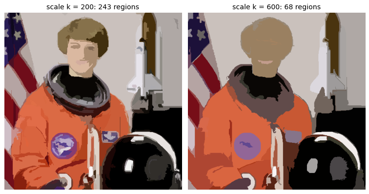
Felzenszwalb and Huttenlocher (2004) treat the image as a graph \(G=(V,E)\): pixels are vertices, edges join neighbors, and each edge weight \(w(e)\) measures dissimilarity (for example the intensity difference between \(N_8\) neighbors). Regions grow by merging, guided by a comparison of within-region and between-region differences.
For a region \(C\), the internal difference is the largest edge in its minimum spanning tree:
The difference between two regions is the lightest edge connecting them:
The minimum internal difference adds a size-dependent penalty \(\tau(C)=k/\lvert C\rvert\) that lets small regions merge more easily:
The merge test compares the two:
Two regions are merged when \(D\) is false, that is when the gap between them is no larger than the variation already inside them. The single parameter \(k\) sets the preferred region scale.
from skimage.segmentation import felzenszwalb

img = util.img_as_float(data.astronaut())
fine   = felzenszwalb(img, scale=200, sigma=0.8, min_size=100)
coarse = felzenszwalb(img, scale=600, sigma=0.8, min_size=200)   # larger k -> fewer, bigger regions

fig, ax = plt.subplots(1, 2, figsize=(9, 4.6))
show(ax[0], color.label2rgb(fine,   img, kind='avg', bg_label=-1),
     f'scale k = 200: {len(np.unique(fine))} regions')
show(ax[1], color.label2rgb(coarse, img, kind='avg', bg_label=-1),
     f'scale k = 600: {len(np.unique(coarse))} regions')
plt.tight_layout(); plt.show()
5. Probabilistic aggregation#
Alpert et al. (2007) merge regions with a probabilistic, bottom-up rule that combines two cues: gray-level similarity and texture similarity. Each pair of neighboring regions \(i,j\) gets a merging likelihood \(p_{ij}\). Starting from one region per pixel, a coarser graph is built by selecting a subset of seed regions \(C\) and absorbing any region that is strongly coupled to them:
The assignment found at a coarse level is propagated back to the finer regions, and the process repeats, giving a multiscale segmentation known as segmentation by weighted aggregation (SWA). This section is concept-only: the merging and splitting mechanics are shown by the demos above and below.
6. Mean shift#
Mean shift (Comaniciu and Meer, 2002) treats each pixel feature (color, or color plus position) as a sample from an unknown density, and segments by finding the modes (peaks) of that density: every pixel that climbs to the same peak forms one region.
The density is estimated by placing a kernel of bandwidth \(h\) on each sample:
Its gradient points toward higher density and rearranges into a weighted-mean form:
where \(G = -k'\). The vector \(m(\mathbf{x})\) is the mean shift: the offset from \(\mathbf{x}\) to the local weighted mean of its neighbors. Following it repeatedly is a gradient ascent that lands on a mode:
No density is ever computed explicitly; each point simply walks uphill to its peak.
rng = np.random.default_rng(1)
pts = np.concatenate([rng.normal(-3, 0.6, 60), rng.normal(2.5, 0.8, 80)])
h   = 0.8
grid = np.linspace(-6, 6, 400)

def kde(x, pts, h):
    u = (np.atleast_1d(x)[:, None] - pts[None, :]) / h
    return np.exp(-0.5 * u**2).sum(1) / (len(pts) * h * np.sqrt(2 * np.pi))

def mean_shift_1d(y, pts, h, iters=100, tol=1e-6):
    traj = [y]
    for _ in range(iters):
        w = np.exp(-0.5 * ((y - pts) / h)**2)
        y_new = (w * pts).sum() / w.sum()
        traj.append(y_new)
        if abs(y_new - y) < tol: break
        y = y_new
    return np.array(traj)

dens   = kde(grid, pts, h)
starts = [-5.0, -1.5, 0.5, 4.5]
trajs  = [mean_shift_1d(s, pts, h) for s in starts]
modes  = sorted(set(round(float(t[-1]), 2) for t in trajs))

fig, ax = plt.subplots(1, 2, figsize=(11, 3.6))
ax[0].plot(grid, dens, color='green')
ax[0].plot(pts, np.full_like(pts, -0.004), '|', color='0.5', markersize=8)   # data rug
for m in modes:
    ax[0].axvline(m, ls='--', color='crimson', lw=1)
    ax[0].plot(m, kde(m, pts, h)[0], 'o', color='crimson')
ax[0].set_title(f'kernel density estimate, modes at {modes}')
ax[0].set_xlabel('feature value'); ax[0].set_yticks([])

for s, t in zip(starts, trajs):
    ax[1].plot(range(len(t)), t, marker='o', ms=3)
for m in modes:
    ax[1].axhline(m, ls='--', color='0.6', lw=1)
ax[1].set_title('mean-shift trajectories (each start climbs to a mode)')
ax[1].set_xlabel('iteration'); ax[1].set_ylabel('estimate')
plt.tight_layout(); plt.show()
print('modes reached:', modes)
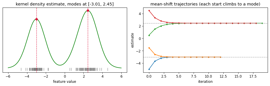
modes reached: [-3.01, 2.45]
rng = np.random.default_rng(2)
clouds = [rng.normal([0, 0], 0.5, (50, 2)),
          rng.normal([3, 3], 0.6, (50, 2)),
          rng.normal([0, 3.5], 0.4, (40, 2))]
P = np.vstack(clouds)
h = 0.9

def mean_shift_point(y, pts, h, iters=200, tol=1e-5):
    for _ in range(iters):
        w = np.exp(-0.5 * ((pts - y)**2).sum(1) / h**2)
        y_new = (w[:, None] * pts).sum(0) / w.sum()
        if np.linalg.norm(y_new - y) < tol: break
        y = y_new
    return y

peaks = np.array([mean_shift_point(p.copy(), P, h) for p in P])

# group points whose peaks coincide -> one label (segment) per mode
labels = -np.ones(len(P), int); centers = []
for i, pk in enumerate(peaks):
    for cid, c in enumerate(centers):
        if np.linalg.norm(pk - c) < 0.5:
            labels[i] = cid; break
    else:
        labels[i] = len(centers); centers.append(pk)
centers = np.array(centers)

# left: 2D clustering by mode, with a few full ascent paths overlaid
fig, ax = plt.subplots(1, 2, figsize=(11, 4.2))
ax[0].scatter(P[:, 0], P[:, 1], c=labels, cmap='tab10', s=25)
for s in np.array([[-1.5, -1.0], [4.0, 4.2], [-1.2, 4.5], [1.5, 1.5]]):
    path = [s.copy()]; y = s.copy()
    for _ in range(60):
        w = np.exp(-0.5 * ((P - y)**2).sum(1) / h**2)
        y = (w[:, None] * P).sum(0) / w.sum(); path.append(y.copy())
    path = np.array(path)
    ax[0].plot(path[:, 0], path[:, 1], '-', color='0.3', lw=1)
ax[0].scatter(centers[:, 0], centers[:, 1], marker='X', s=180,
              c='k', edgecolors='w', linewidths=1.5, zorder=5)
ax[0].set_title(f'2D mean shift: {len(centers)} modes = {len(centers)} segments')
ax[0].set_aspect('equal'); ax[0].set_xticks([]); ax[0].set_yticks([])

# right: the same idea on real pixels, via OpenCV mean-shift filtering
img = util.img_as_float(data.astronaut())[::2, ::2]
bgr = cv2.cvtColor(to_u8(img), cv2.COLOR_RGB2BGR)
flat = cv2.cvtColor(cv2.pyrMeanShiftFiltering(bgr, sp=20, sr=35), cv2.COLOR_BGR2RGB)
show(ax[1], flat, 'image after mean-shift filtering (flattened regions)')
plt.tight_layout(); plt.show()

n0 = len(np.unique(to_u8(img).reshape(-1, 3), axis=0))
n1 = len(np.unique(flat.reshape(-1, 3), axis=0))
print(f'unique colors {n0} -> {n1} after mean shift')
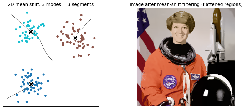
unique colors 38111 -> 9184 after mean shift
7. Normalized cuts#
Segmentation can also be posed as graph splitting. Build a graph where edge weights \(w_{ij}\) encode pixel similarity, and cut it into two parts \(A\) and \(B\). The weight removed is the cut:
Minimizing the cut directly has a well-known failure: the cheapest cut often just peels off a single isolated pixel. Shi and Malik (2000) fix this by normalizing the cut by how strongly each side connects to the whole graph. With
the normalized cut is
Dividing by the association penalizes tiny fragments, so the split is balanced. The exact optimum is NP-complete, but a good approximation comes from a spectral relaxation: solve the generalized eigenproblem \((D-W)\,\mathbf{y} = \lambda\, D\,\mathbf{y}\) and threshold the eigenvector of the second-smallest eigenvalue (the Fiedler vector), where \(W\) is the affinity matrix and \(D\) its diagonal degree matrix.
from scipy.linalg import eigh

rng = np.random.default_rng(3)
A = rng.normal([0, 0], 0.45, (25, 2))
B = rng.normal([3, 0.3], 0.5, (25, 2))
outlier = np.array([[6.0, 3.0]])                       # one far, weakly connected point
pts = np.vstack([A, B, outlier])

d2 = ((pts[:, None, :] - pts[None, :, :])**2).sum(-1)
W  = np.exp(-d2 / (2 * 1.0**2)); np.fill_diagonal(W, 0)
D  = np.diag(W.sum(1))

# spectral Ncut: Fiedler vector of the generalized eigenproblem, then threshold at 0
_, vecs = eigh(D - W, D)
ncut_label = (vecs[:, 1] > 0).astype(int)

# raw min-cut proxy: the cheapest single-node cut removes the least-connected point
mincut_label = np.zeros(len(pts), int)
mincut_label[np.argmin(W.sum(1))] = 1                  # that node is the outlier

fig, ax = plt.subplots(1, 2, figsize=(11, 4.2))
ax[0].scatter(pts[:, 0], pts[:, 1], c=mincut_label, cmap='coolwarm', s=35, edgecolors='0.3')
ax[0].set_title('min-cut criterion: isolates one point (trivial)')
ax[1].scatter(pts[:, 0], pts[:, 1], c=ncut_label, cmap='coolwarm', s=35, edgecolors='0.3')
ax[1].set_title('normalized cut: balanced two-way split')
for a in ax: a.set_aspect('equal'); a.set_xticks([]); a.set_yticks([])
plt.tight_layout(); plt.show()
print('Ncut split sizes:', np.bincount(ncut_label))
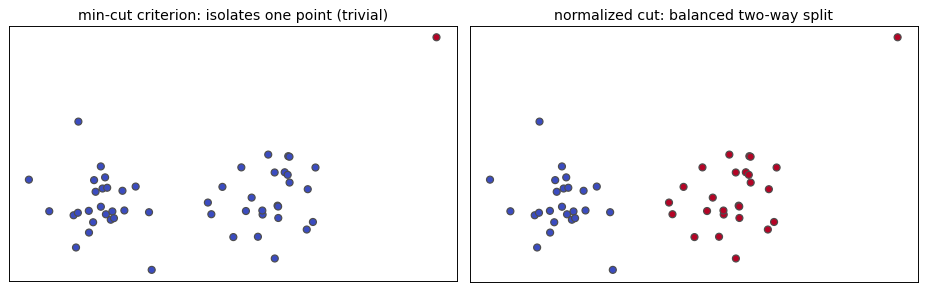
Ncut split sizes: [25 26]
8. Other methods and beyond images#
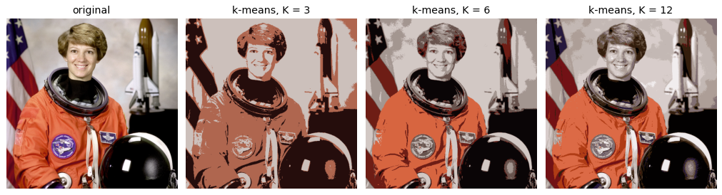
Many more segmentation methods exist, including k-means clustering in color space and Markov / Conditional Random Fields that add spatial smoothness priors. k-means is the simplest: pick \(K\), cluster the pixel colors, and recolor each pixel by its cluster center.
Do we still need these with deep learning? To an extent, yes. Classical segmentation shaped early deep pipelines: the first R-CNN used a min-cut variant, Constrained Parametric Min-Cuts, to propose regions. These ideas also extend beyond single images: shot boundary detection splits a video into shots by finding frames where appearance changes abruptly, and motion segmentation isolates moving objects.
img = util.img_as_float(data.astronaut())
Z = img.reshape(-1, 3).astype(np.float32)
crit = (cv2.TERM_CRITERIA_EPS + cv2.TERM_CRITERIA_MAX_ITER, 20, 1.0)

fig, ax = plt.subplots(1, 4, figsize=(12, 3.2))
show(ax[0], img, 'original')
for a, K in zip(ax[1:], [3, 6, 12]):
    _, lab, ctr = cv2.kmeans(Z, K, None, crit, 5, cv2.KMEANS_PP_CENTERS)
    quant = np.clip(ctr[lab.flatten()].reshape(img.shape), 0, 1)
    show(a, quant, f'k-means, K = {K}')
plt.tight_layout(); plt.show()
rng = np.random.default_rng(4)
def jitter(base, amp=6):
    return np.clip(base + rng.integers(-amp, amp, base.shape), 0, 255).astype(np.uint8)

scene_a = rng.integers(30, 90,  (64, 64)).astype(np.uint8)
scene_b = rng.integers(120, 200, (64, 64)).astype(np.uint8)
frames  = [jitter(scene_a) for _ in range(8)] + [jitter(scene_b) for _ in range(8)]

def hist(f):
    h, _ = np.histogram(f, bins=32, range=(0, 255)); return h / h.sum()

diffs = np.array([np.abs(hist(frames[i]) - hist(frames[i - 1])).sum()
                  for i in range(1, len(frames))])
boundary = int(np.argmax(diffs)) + 1                 # frame index where the shot changes

sep = np.full((64, 2), 255, np.uint8)
strip = frames[0]
for f in frames[1:]:
    strip = np.hstack([strip, sep, f])

fig, ax = plt.subplots(2, 1, figsize=(11, 4.2), gridspec_kw={'height_ratios': [1, 1.2]})
ax[0].imshow(strip, cmap='gray'); ax[0].axis('off')
ax[0].axvline(boundary * 66 - 1, color='crimson', lw=2)
ax[0].set_title('16-frame clip: two shots (boundary in red)')
ax[1].plot(range(1, len(frames)), diffs, marker='o')
ax[1].plot(boundary, diffs[boundary - 1], 'o', color='crimson', ms=10)
ax[1].set_title(f'histogram difference spikes at the cut (frame {boundary})')
ax[1].set_xlabel('frame'); ax[1].set_ylabel('L1 histogram diff')
plt.tight_layout(); plt.show()
print('detected shot boundary before frame', boundary)
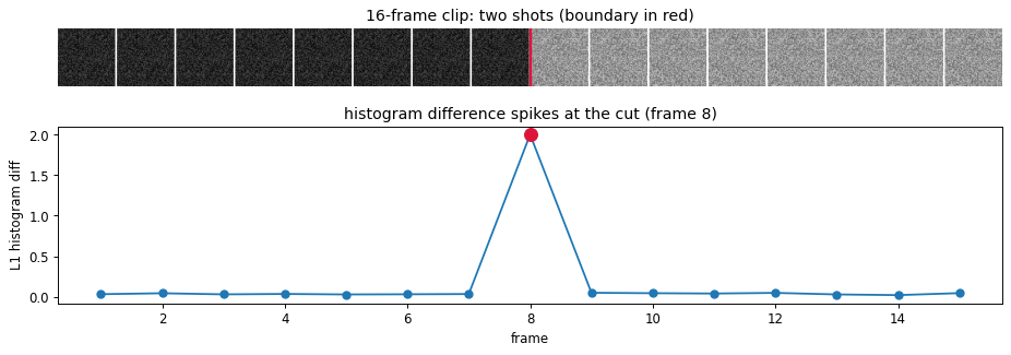
detected shot boundary before frame 8
9. Explore and verify#
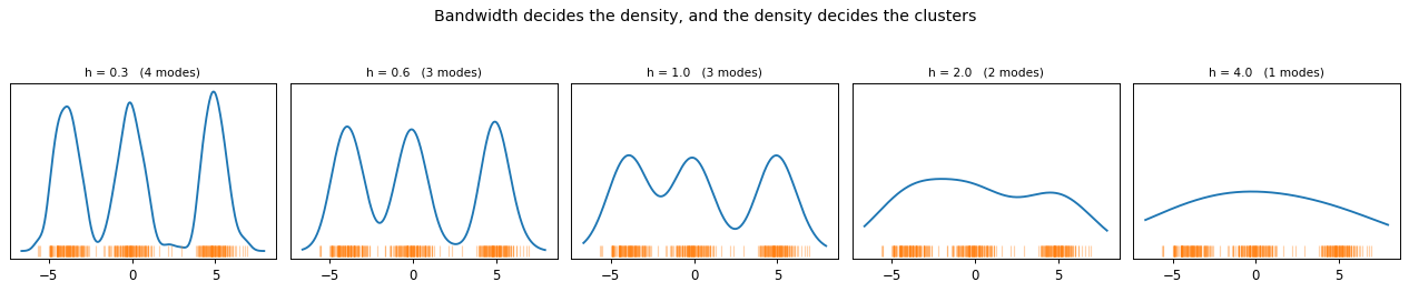
Mean shift has one parameter, the bandwidth, and the lecture claims it alone decides how many modes you find. That is a claim we can measure: sweep the bandwidth and count.
# Verify the bandwidth claim.  mean_shift_1d returns the whole trajectory; the mode is [-1].
rng = np.random.default_rng(0)
pts = np.concatenate([rng.normal(-4, 0.7, 120), rng.normal(0, 0.7, 120), rng.normal(5, 0.7, 120)])

def count_modes(h, tol=0.25):
    modes = [mean_shift_1d(y, pts, h)[-1] for y in np.linspace(pts.min(), pts.max(), 60)]
    uniq = []
    for m in sorted(modes):
        if not uniq or abs(m - uniq[-1]) > tol:
            uniq.append(m)
    return len(uniq)

counts = [(h, count_modes(h)) for h in (0.3, 0.6, 1.0, 2.0, 4.0)]
for h, c in counts:
    print(f'  bandwidth {h:4.1f}  ->  {c} modes')

seq = [c for _, c in counts]
assert seq == sorted(seq, reverse=True), f'mode count is not monotone in bandwidth: {seq}'
assert seq[-1] == 1, 'a very wide bandwidth should collapse to a single mode'
print(f'\nmode count falls monotonically with bandwidth: {seq}')
print('the data really has 3 clusters; only a well-chosen bandwidth recovers them')
  bandwidth  0.3  ->  4 modes
  bandwidth  0.6  ->  3 modes
  bandwidth  1.0  ->  3 modes
  bandwidth  2.0  ->  2 modes
  bandwidth  4.0  ->  1 modes

mode count falls monotonically with bandwidth: [4, 3, 3, 2, 1]
the data really has 3 clusters; only a well-chosen bandwidth recovers them
# Static sweep: the KDE that mean shift is climbing. kde() is already vectorized over x.
grid = np.linspace(pts.min() - 1, pts.max() + 1, 400)

fig, ax = plt.subplots(1, 5, figsize=(15, 2.9), sharey=True)
for a, h in zip(ax, [0.3, 0.6, 1.0, 2.0, 4.0]):
    a.plot(grid, kde(grid, pts, h), lw=1.6)
    a.plot(pts, np.zeros_like(pts), '|', ms=8, alpha=0.35)
    a.set_title(f'h = {h}   ({count_modes(h)} modes)', fontsize=9)
    a.set_yticks([])
fig.suptitle('Bandwidth decides the density, and the density decides the clusters', y=1.05)
plt.tight_layout(); plt.show()
Now the same thing under your control. Drag the slider and watch what changes.
# Live: choose the bandwidth yourself.
from ipywidgets import interact, FloatSlider

def ms(h=1.0):
    fig, a = plt.subplots(figsize=(7.5, 3.2))
    a.plot(grid, kde(grid, pts, h), lw=1.8)
    a.plot(pts, np.zeros_like(pts), '|', ms=9, alpha=0.35)
    a.set_yticks([]); a.set_title(f'bandwidth h = {h:.2f}  ->  {count_modes(h)} modes')
    plt.tight_layout(); plt.show()

interact(ms, h=FloatSlider(min=0.2, max=4.0, step=0.1, value=1.0, description='bandwidth'));
Key takeaways#
Method |
Core idea |
|---|---|
Gestalt grouping |
Perceptual cues (proximity, similarity, closure, and more) that motivate grouping; descriptive, not algorithmic |
Watershed |
Flood the intensity or gradient surface from minima; basins are regions, ridges are boundaries; markers avoid over-segmentation |
Superpixels (SLIC) |
Localized k-means in color-plus-position space; compact regions used as preprocessing |
Graph-based (Felzenszwalb) |
Merge two regions when the between-region gap is no larger than the within-region variation (\(\mathrm{Dif} \le \mathrm{MInt}\)) |
Probabilistic aggregation |
Bottom-up SWA merging using gray and texture coupling above a threshold |
Mean shift |
Climb the feature-density gradient to a mode; pixels sharing a mode share a region |
Normalized cuts |
Balanced graph split minimizing \(\mathrm{Ncut}\); spectral relaxation via the Fiedler vector |
k-means, MRF and CRF |
Color clustering; random-field models add spatial smoothness |
Reading: Szeliski, Computer Vision: Algorithms and Applications, Chapter 5. Forsyth and Ponce, Computer Vision: A Modern Approach, Chapters 15 and 17. Shi and Malik, Normalized Cuts and Image Segmentation, IEEE TPAMI 2000. Comaniciu and Meer, Mean Shift, IEEE TPAMI 2002.
To think about: Why does the raw min-cut criterion favor tiny isolated regions, and how does normalization repair it? How does the mean-shift bandwidth \(h\) trade the number of regions against detail? Derive the mean-shift update from the gradient of the kernel density (lecture homework). Which of these classical ideas can you still spot inside a modern segmentation network?
Exercises#
Markers tame watershed. Run watershed on a gradient image with and without markers, and count regions. Explain the over-segmentation that markers remove.
SLIC compactness. Sweep the compactness parameter and describe the trade-off between regions that follow boundaries and regions that stay compact.
Felzenszwalb’s scale. Sweep the scale parameter and relate what you see to the merge rule \(\mathrm{Dif} \le \mathrm{MInt}\).
Bandwidth sets the mode count. Sweep the mean shift bandwidth and plot the number of modes found. Why is this parameter harder to set than \(k\) in k-means?