
📺 Lecture video | 📄 Slides
Week 3, Lecture 2: The XOR Conundrum, MLPs, and Activation Functions#
NPTEL Deep Learning for Computer Vision | Prof. Vineeth N Balasubramanian, IIT Hyderabad
Companion notebook for §3.1 Neural Networks: A Review.
A single perceptron can draw only one straight line, so it cannot solve XOR. In this notebook we see exactly why, then watch a hidden layer bend the space so that XOR becomes easy. Along the way we meet smooth activation functions and the Universal Approximation Theorem.
What you will learn
Why XOR is not linearly separable: the four perceptron inequalities contradict each other.
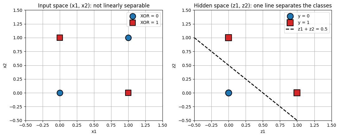
How a Multi-Layer Perceptron (MLP) remaps the inputs into a hidden space where XOR is linearly separable (the key “aha”).
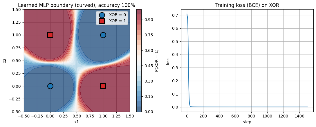
Training an MLP on XOR in PyTorch and plotting its curved decision boundary.
An activation zoo built from scratch (step, sigmoid, tanh, ReLU, Leaky ReLU, ELU) with their derivatives, and why a smooth sigmoid replaced the harsh step.
A hands-on Universal Approximation demo: one hidden layer of neurons fitting a wiggly 1D function.
How to run
Runs on Google Colab (CPU or GPU) or local Jupyter. No downloads, no external files.
Run the setup cell first, then the cells top to bottom. Every cell finishes in a few seconds on CPU.
The interactive sliders use
ipywidgets. If a widget does not render, run its cell again.
Contents
The XOR conundrum, one line is not enough
A hidden layer makes XOR linearly separable (the “aha”)
Let PyTorch learn the hidden layer
The activation zoo (built from scratch)
Universal Approximation in action
Review#
The previous lecture built the McCulloch-Pitts neuron and the Perceptron, and watched the Perceptron Learning Algorithm converge on linearly separable data. That last qualifier is the catch, and this lecture starts with a problem no single perceptron can solve.
Setup#
# Run this cell first. Works on Colab (CPU or GPU) and local Jupyter.
import sys, subprocess
# ipywidgets ships with Colab; install only if it is missing.
try:
    import ipywidgets  # noqa: F401
except ImportError:
    subprocess.run([sys.executable, "-m", "pip", "install", "-q", "ipywidgets"])

import numpy as np
import torch
import torch.nn as nn
import torch.nn.functional as F
import matplotlib.pyplot as plt
from ipywidgets import interact, interactive, FloatSlider, IntSlider, Dropdown, Checkbox, fixed
%matplotlib inline

# Reproducibility
torch.manual_seed(0)
np.random.seed(0)

# Use a GPU if one is available, otherwise CPU. Every demo here is tiny and
# runs in seconds on CPU, so no GPU is required.
device = torch.device("cuda" if torch.cuda.is_available() else "cpu")

plt.rcParams["figure.figsize"] = (7, 4.5)
plt.rcParams["axes.grid"] = True
plt.rcParams["axes.axisbelow"] = True

print("PyTorch", torch.__version__, "| device:", device)
PyTorch 2.8.0 | device: cpu
1. The XOR conundrum, one line is not enough#
XOR (exclusive OR) outputs 1 when exactly one input is 1:
\(x_1\) |
\(x_2\) |
XOR |
|---|---|---|
0 |
0 |
0 |
0 |
1 |
1 |
1 |
0 |
1 |
1 |
1 |
0 |
A single perceptron predicts \(1\) when \(w_0 + w_1 x_1 + w_2 x_2 \ge 0\) and \(0\) otherwise, so it splits the plane with one straight line. Forcing that line to match all four XOR rows gives four inequalities (this is the slide’s derivation):
\((0,0)\to 0:\quad w_0 < 0\)
\((1,0)\to 1:\quad w_1 > -w_0\)
\((0,1)\to 1:\quad w_2 > -w_0\)
\((1,1)\to 0:\quad w_1 + w_2 < -w_0\)
Add inequalities 2 and 3: \(w_1 + w_2 > -2w_0\). Since \(w_0 < 0\) we have \(-2w_0 > -w_0 > 0\), hence \(w_1 + w_2 > -w_0\). That directly contradicts inequality 4. No weights satisfy all four at once, so no single line separates XOR.
# The four XOR points and their target labels (kept on `device`).
X_xor = torch.tensor([[0., 0.],
                      [0., 1.],
                      [1., 0.],
                      [1., 1.]], device=device)
y_xor = torch.tensor([0., 1., 1., 0.], device=device)  # XOR of the two inputs

print("XOR truth table")
for (a, b), t in zip(X_xor.tolist(), y_xor.tolist()):
    print(f"  x1={int(a)}  x2={int(b)}  ->  XOR={int(t)}")
XOR truth table
  x1=0  x2=0  ->  XOR=0
  x1=0  x2=1  ->  XOR=1
  x1=1  x2=0  ->  XOR=1
  x1=1  x2=1  ->  XOR=0
Two small plotting helpers#
We reuse these in Parts 1, 2, and 3: one scatters the XOR points colored by label, the
other shades a model’s decision region on a grid (a contourf mesh).
def plot_xor_points(ax):
    """Scatter the 4 XOR points: blue circles for label 0, red squares for label 1."""
    Xn, yn = X_xor.cpu().numpy(), y_xor.cpu().numpy()
    for cls, marker, color, name in [(0, "o", "tab:blue", "XOR = 0"),
                                     (1, "s", "tab:red", "XOR = 1")]:
        m = yn == cls
        ax.scatter(Xn[m, 0], Xn[m, 1], c=color, marker=marker, s=180,
                   edgecolors="k", linewidths=1.5, zorder=3, label=name)

def decision_surface(ax, predict_fn, lo=-0.5, hi=1.5, steps=200):
    """Shade P(label = 1) over a grid using the model's probability output."""
    xs = np.linspace(lo, hi, steps)
    ys = np.linspace(lo, hi, steps)
    gx, gy = np.meshgrid(xs, ys)
    grid = np.stack([gx.ravel(), gy.ravel()], axis=1)
    with torch.no_grad():
        g = torch.tensor(grid, dtype=torch.float32, device=device)
        z = predict_fn(g).view(gx.shape).cpu().numpy()
    cs = ax.contourf(gx, gy, z, levels=np.linspace(0, 1, 21), cmap="RdBu_r", alpha=0.7)
    ax.set_xlim(lo, hi)
    ax.set_ylim(lo, hi)
    return cs
# Try to fit XOR with a single perceptron: one linear unit followed by a sigmoid.
torch.manual_seed(0)
perceptron = nn.Sequential(nn.Linear(2, 1), nn.Sigmoid()).to(device)
opt = torch.optim.Adam(perceptron.parameters(), lr=0.1)
loss_fn = nn.BCELoss()
target = y_xor.view(-1, 1)

for step_i in range(500):
    opt.zero_grad()
    loss = loss_fn(perceptron(X_xor), target)
    loss.backward()
    opt.step()

with torch.no_grad():
    probs = perceptron(X_xor).view(-1)
    preds = (probs >= 0.5).float()
    acc = (preds == y_xor).float().mean().item()

print(f"Final BCE loss: {loss.item():.3f}")
print(f"Output probabilities: {[round(p, 3) for p in probs.tolist()]}")
print(f"Predicted labels:     {preds.tolist()}")
print(f"True XOR labels:      {y_xor.tolist()}")
print(f"Accuracy of the best single line: {acc*100:.0f}%")
Final BCE loss: 0.693
Output probabilities: [0.5, 0.5, 0.5, 0.5]
Predicted labels:     [1.0, 1.0, 1.0, 1.0]
True XOR labels:      [0.0, 1.0, 1.0, 0.0]
Accuracy of the best single line: 50%
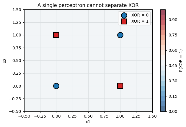
The best any single line can do on XOR is 3 of 4 correct. Here gradient descent does something even more telling: it collapses to outputting about \(0.5\) for every point (loss \(\approx \ln 2 = 0.693\)). Unable to separate the classes, the perceptron simply hedges. The plot below shades \(P(\text{XOR}=1)\): an almost uniform field with no real boundary.
fig, ax = plt.subplots()
cs = decision_surface(ax, lambda g: perceptron(g).view(-1))
plot_xor_points(ax)
fig.colorbar(cs, ax=ax, label="P(XOR = 1)")
ax.set_title("A single perceptron cannot separate XOR")
ax.set_xlabel("x1")
ax.set_ylabel("x2")
ax.legend(loc="upper right")
plt.show()
Widget 1: try to separate XOR by hand#
Move the sliders for \(w_0, w_1, w_2\). The dashed line is the decision boundary \(w_0 + w_1 x_1 + w_2 x_2 = 0\), shaded red where the perceptron predicts 1. The title reports how many of the four points you got right. The default is the OR line, which scores 3 of 4. Try as you like: you will never reach 4 of 4.
def try_linear_boundary(w0=-0.5, w1=1.0, w2=1.0):
    Xn, yn = X_xor.cpu().numpy(), y_xor.cpu().numpy()
    score = w0 + w1 * Xn[:, 0] + w2 * Xn[:, 1]
    pred = (score >= 0).astype(float)
    n_correct = int((pred == yn).sum())

    xs = np.linspace(-0.5, 1.5, 200)
    gx, gy = np.meshgrid(xs, xs)
    region = (w0 + w1 * gx + w2 * gy >= 0).astype(float)

    fig, ax = plt.subplots()
    ax.contourf(gx, gy, region, levels=[-0.5, 0.5, 1.5], cmap="RdBu_r", alpha=0.5)
    if abs(w2) > 1e-6:
        ax.plot(xs, -(w0 + w1 * xs) / w2, "k--", lw=2, label="decision line")
    plot_xor_points(ax)
    ax.set_xlim(-0.5, 1.5)
    ax.set_ylim(-0.5, 1.5)
    ax.set_title(f"Your line gets {n_correct} of 4 XOR points correct (best possible = 3)")
    ax.set_xlabel("x1")
    ax.set_ylabel("x2")
    ax.legend(loc="upper right")
    plt.show()

interact(try_linear_boundary,
         w0=FloatSlider(min=-3.0, max=3.0, step=0.1, value=-0.5),
         w1=FloatSlider(min=-3.0, max=3.0, step=0.1, value=1.0),
         w2=FloatSlider(min=-3.0, max=3.0, step=0.1, value=1.0));
4. The activation zoo (built from scratch)#
The sigmoid keeps the S shape of the step but is smooth, continuous, and differentiable, with output in \((0,1)\) that reads as a probability: $\( \sigma(z) = \frac{1}{1 + e^{-z}}, \qquad z = w_0 + \sum_i w_i x_i. \)$
We implement each activation from scratch with torch, then let autograd compute its derivative. Definitions from the slide (with \(z = \sum_i w_i x_i\)):
Sigmoid: \(\sigma(z) = 1/(1+e^{-z})\)
Tanh: \(\tanh(z) = (e^{z}-e^{-z})/(e^{z}+e^{-z})\)
ReLU: \(\max(0, z)\)
Leaky ReLU: \(\max(\alpha z, z)\), with small \(\alpha \in (0,1)\)
ELU: \(z\) for \(z>0\), else \(\alpha(e^{z}-1)\), with \(\alpha>0\)
Why this matters: the step has derivative \(0\) almost everywhere (and undefined at the jump), so it carries no gradient signal. Every function below except the step has a useful, nonzero derivative, which is what makes gradient based learning possible.
# The activation zoo, from scratch with torch ops.
def step_act(z):        return (z >= 0).float()
def sigmoid_act(z):     return 1.0 / (1.0 + torch.exp(-z))
def tanh_act(z):        return (torch.exp(z) - torch.exp(-z)) / (torch.exp(z) + torch.exp(-z))
def relu_act(z):        return torch.clamp(z, min=0.0)              # max(0, z)
def leaky_relu_act(z, alpha=0.1):  return torch.maximum(alpha * z, z)
def elu_act(z, alpha=1.0):         return torch.where(z > 0, z, alpha * (torch.exp(z) - 1.0))

def deriv(fn, z):
    """Derivative of an activation via autograd. Step is flat, so its gradient is 0."""
    zz = z.clone().detach().requires_grad_(True)
    y = fn(zz)
    if not y.requires_grad:          # step: no grad_fn, derivative is 0 almost everywhere
        return torch.zeros_like(z)
    g, = torch.autograd.grad(y.sum(), zz)
    return g.detach()

# Sanity check against tanh's known derivative 1 - tanh(z)^2.
zc = torch.linspace(-2, 2, 5, device=device)
print("autograd d/dz tanh:", [round(v, 3) for v in deriv(tanh_act, zc).tolist()])
print("formula 1 - tanh^2:", [round(v, 3) for v in (1 - tanh_act(zc) ** 2).tolist()])
autograd d/dz tanh: [0.071, 0.42, 1.0, 0.42, 0.071]
formula 1 - tanh^2: [0.071, 0.42, 1.0, 0.42, 0.071]
z = torch.linspace(-4, 4, 400, device=device)
zoo = [("step", step_act), ("sigmoid", sigmoid_act), ("tanh", tanh_act),
       ("ReLU", relu_act), ("Leaky ReLU", leaky_relu_act), ("ELU", elu_act)]

fig, axes = plt.subplots(2, 3, figsize=(12, 7))
zc = z.cpu().numpy()
for ax, (name, fn) in zip(axes.ravel(), zoo):
    ax.plot(zc, fn(z).detach().cpu().numpy(), lw=2, label=name)
    ax.plot(zc, deriv(fn, z).cpu().numpy(), "--", lw=2, label="derivative")
    ax.axhline(0, color="gray", lw=0.8)
    ax.axvline(0, color="gray", lw=0.8)
    ax.set_title(name)
    ax.set_xlabel("z")
    ax.set_ylabel("value")
    ax.legend(loc="upper left", fontsize=8)

fig.suptitle("Activation functions (solid) and their derivatives (dashed)")
plt.tight_layout()
plt.show()
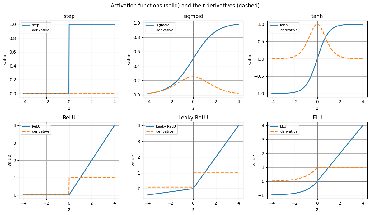
Notice the contrast: the step has a derivative that is flat at 0 (no learning signal), while sigmoid and tanh have smooth bell-shaped derivatives. ReLU and Leaky ReLU are piecewise linear with a kink at 0 where the slope jumps; Leaky ReLU keeps a small slope \(\alpha\) for negative inputs so those units never fully die. ELU smooths the negative side with an exponential.
Widget 3: explore one activation and its parameter#
Pick an activation and adjust its parameter: the sigmoid gain (steepness), the Leaky ReLU slope \(\alpha\), or the ELU \(\alpha\). The function and its derivative redraw together. Push the sigmoid gain up and watch it approach the harsh step (and its derivative shrink toward a spike): that is exactly the behavior we wanted to avoid.
def activation_explorer(activation="sigmoid", sigmoid_gain=1.0, leaky_alpha=0.1, elu_alpha=1.0):
    if activation == "step":
        f = lambda t: step_act(t)
    elif activation == "sigmoid":
        f = lambda t: sigmoid_act(sigmoid_gain * t)
    elif activation == "tanh":
        f = lambda t: tanh_act(t)
    elif activation == "ReLU":
        f = lambda t: relu_act(t)
    elif activation == "Leaky ReLU":
        f = lambda t: leaky_relu_act(t, leaky_alpha)
    else:  # ELU
        f = lambda t: elu_act(t, elu_alpha)

    zt = torch.linspace(-4, 4, 400, device=device)
    zn = zt.cpu().numpy()
    fig, ax = plt.subplots()
    ax.plot(zn, f(zt).detach().cpu().numpy(), lw=2, label=activation)
    ax.plot(zn, deriv(f, zt).cpu().numpy(), "--", lw=2, label="derivative")
    ax.axhline(0, color="gray", lw=0.8)
    ax.axvline(0, color="gray", lw=0.8)
    ax.set_ylim(-1.6, 4.2)
    ax.set_title(f"{activation}: function (solid) and derivative (dashed)")
    ax.set_xlabel("z")
    ax.set_ylabel("value")
    ax.legend(loc="upper left")
    plt.show()

interact(activation_explorer,
         activation=Dropdown(options=["step", "sigmoid", "tanh", "ReLU", "Leaky ReLU", "ELU"],
                             value="sigmoid"),
         sigmoid_gain=FloatSlider(min=0.5, max=8.0, step=0.5, value=1.0),
         leaky_alpha=FloatSlider(min=0.0, max=0.5, step=0.01, value=0.1),
         elu_alpha=FloatSlider(min=0.1, max=2.0, step=0.1, value=1.0));
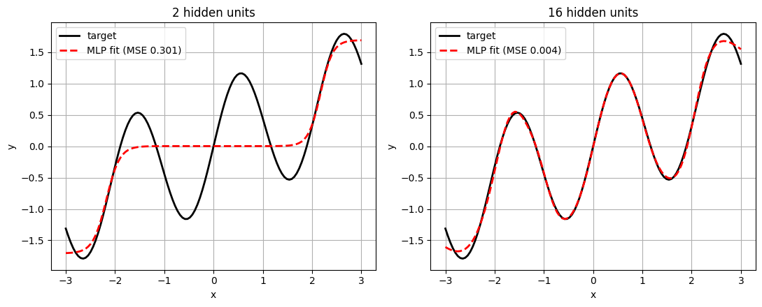
5. Universal Approximation in action#
Theorem (Cybenko 1989; Hornik et al. 1989). A network with a single hidden layer of sigmoid neurons can approximate any continuous function to any desired precision, given enough hidden units.
We test this on a wiggly 1D target \(f(x) = \sin(3x) + 0.3x\). A one hidden layer MLP
(Linear -> Tanh -> Linear) is trained briefly (tanh is a shifted, scaled sigmoid, so the
theorem still applies and it trains a little faster). As we add hidden units, the fit
visibly tightens: more units means more little bumps the network can add up to trace the
curve.
def target_fn(x):
    return torch.sin(3.0 * x) + 0.3 * x

x_train = torch.linspace(-3, 3, 120, device=device).view(-1, 1)
y_train = target_fn(x_train)

def fit_1d(hidden=16, steps=600, lr=0.05, seed=0):
    torch.manual_seed(seed)
    net = nn.Sequential(nn.Linear(1, hidden), nn.Tanh(), nn.Linear(hidden, 1)).to(device)
    opt = torch.optim.Adam(net.parameters(), lr=lr)
    loss_fn = nn.MSELoss()
    for _ in range(steps):
        opt.zero_grad()
        loss = loss_fn(net(x_train), y_train)
        loss.backward()
        opt.step()
    return net, loss.item()

# Too few units underfits; enough units traces the curve.
fig, axes = plt.subplots(1, 2, figsize=(11, 4.5))
xc = x_train.cpu().numpy().ravel()
yc = y_train.cpu().numpy().ravel()
for ax, h in zip(axes, [2, 16]):
    net, final_mse = fit_1d(hidden=h, steps=600)
    with torch.no_grad():
        yp = net(x_train).cpu().numpy().ravel()
    ax.plot(xc, yc, "k-", lw=2, label="target")
    ax.plot(xc, yp, "r--", lw=2, label=f"MLP fit (MSE {final_mse:.3f})")
    ax.set_title(f"{h} hidden units")
    ax.set_xlabel("x"); ax.set_ylabel("y")
    ax.legend(loc="upper left")
plt.tight_layout()
plt.show()
Key takeaways#
A single perceptron draws one straight line, so it cannot separate XOR: the four required inequalities contradict each other, and gradient descent just hedges at \(0.5\).
A hidden layer remaps the inputs into a new space where the classes become linearly separable. This is the core idea of a Multi-Layer Perceptron.
Any Boolean function of \(n\) inputs can be represented by one hidden layer of \(2^n\) perceptrons plus an output unit (sufficient, not necessary; the count grows exponentially, so we prefer smaller learned networks).
The step activation is harsh and has zero gradient almost everywhere. Smooth activations (sigmoid, tanh, ReLU, Leaky ReLU, ELU) are differentiable, which is what makes gradient based learning possible.
Universal Approximation (Cybenko 1989; Hornik 1989): one hidden layer of sigmoid neurons can approximate any continuous function to any precision, given enough units.
Exercises#
Solve XOR with an MLP using 4 hidden units (per the lecture slide). Reuse section 3’s
build_and_train_xor(hidden=4, activation=...), try different activations, and check whether it reaches 100%. Which activation and how many steps converge most reliably?