📺 Lecture video  |  📄 Slides

Watch on YouTube

Week 1, Lecture 7: Image Sampling and Interpolation

NPTEL Deep Learning for Computer Vision | Prof. Vineeth N Balasubramanian, IIT Hyderabad

Companion notebook for §1.7 Sampling and Interpolation.

What you will learn

• Compare the cost of convolution in the spatial and frequency domains.

• Sub-sample an image and see aliasing, in 1D against the Nyquist rate and in 2D as moire patterns.

• Prevent aliasing by pre-filtering before sub-sampling.

• Build a Gaussian pyramid.

• Upsample by treating interpolation as convolution, and compare nearest, bilinear and bicubic.

Contents

1. The cost of convolution: spatial vs frequency

2. Sub-sampling

3. Aliasing in 1D and the Nyquist rate

4. Aliasing in 2D: moire patterns

5. Anti-aliasing by pre-filtering

6. The Gaussian pyramid

7. Upsampling: interpolation as convolution

8. Interpolation in practice: nearest, bilinear, bicubic

How to run Runs on Colab or a local Jupyter, CPU only. Every image is bundled with scikit-image, so nothing is downloaded. Run the setup cell first, then go top to bottom.

Review

The previous lecture showed that convolution in space is multiplication in frequency, \(\mathcal{F}[g*h] = \mathcal{F}[g]\mathcal{F}[h]\), which already hints at a cost saving for large kernels. This lecture pushes on the sampling grid itself. Reducing resolution (sub-sampling) and increasing it (interpolation) are everywhere in vision, from image pyramids to the strided and transposed convolutions inside networks, and both go wrong in characteristic ways unless we respect the frequency content of the signal.

Setup

Everything uses images bundled with scikit-image, so the notebook runs offline.

%matplotlib inline
import numpy as np
import matplotlib.pyplot as plt
from scipy import ndimage
from skimage import data, util, color
from skimage.transform import resize

np.random.seed(0)
plt.rcParams['figure.figsize'] = (10, 4)
plt.rcParams['image.cmap']     = 'gray'
plt.rcParams['figure.dpi']     = 85

def load_gray(image, size=None):
    # float grayscale image, optionally resized to (size, size)
    g = color.rgb2gray(image) if image.ndim == 3 else util.img_as_float(image)
    if size is not None:
        g = resize(g, (size, size))
    return g

def show(ax, im, title='', spectrum=False):
    ax.imshow(im, cmap='magma' if spectrum else 'gray')
    ax.set_title(title); ax.axis('off')

1. The cost of convolution: spatial vs frequency

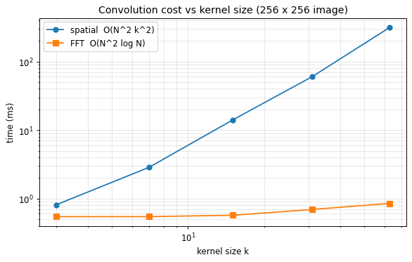
Direct convolution of an \(N \times N\) image with a \(k \times k\) kernel costs \(O(N^2 k^2)\). The convolution theorem replaces this with two FFTs and a pointwise product, costing about \(O(N^2 \log N^2 + k^2 \log k^2)\), which is independent of \(k\) once the image is transformed. So the spatial route wins for tiny kernels (the FFT has fixed overhead) and the frequency route wins as the kernel grows. The crossover is clear in the timings.

import time
from scipy.signal import convolve2d, fftconvolve

img = data.camera().astype(float)[::2, ::2]      # 256 x 256, keeps timing quick
fftconvolve(img, np.ones((3, 3)))                # warm-up so the first timed call is fair

ks, spatial_t, fft_t = [3, 7, 15, 31, 63], [], []
for k in ks:
    ker = np.ones((k, k)) / (k*k)
    t0 = time.perf_counter(); convolve2d(img, ker, mode='same', boundary='symm'); spatial_t.append(time.perf_counter()-t0)
    t0 = time.perf_counter(); fftconvolve(img, ker, mode='same');                 fft_t.append(time.perf_counter()-t0)

plt.figure(figsize=(7, 4.5))
plt.loglog(ks, np.array(spatial_t)*1e3, 'o-', label='spatial  O(N^2 k^2)')
plt.loglog(ks, np.array(fft_t)*1e3,     's-', label='FFT  O(N^2 log N)')
plt.xlabel('kernel size k'); plt.ylabel('time (ms)')
plt.title('Convolution cost vs kernel size (256 x 256 image)')
plt.legend(); plt.grid(True, which='both', alpha=0.3)
plt.tight_layout(); plt.show()

2. Sub-sampling

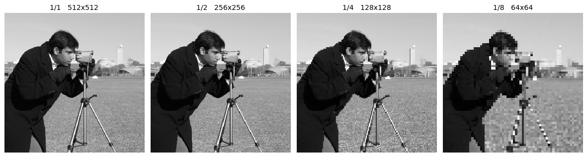
The simplest way to shrink an image is to throw away every other row and column. Repeating this gives the \(1/2\), \(1/4\), \(1/8\) versions below. The result quickly looks broken: thin structures flicker in and out and edges turn jagged. The pixels we keep are not a fair summary of the ones we discard, and the next sections explain why.

img = load_gray(data.camera())
fig, ax = plt.subplots(1, 4, figsize=(14, 4))
for a, s in zip(ax, [1, 2, 4, 8]):
    sub = img[::s, ::s]
    a.imshow(sub, interpolation='nearest')      # nearest keeps the true (aliased) pixels visible
    a.set_title(f'1/{s}   {sub.shape[0]}x{sub.shape[1]}'); a.axis('off')
plt.tight_layout(); plt.show()

3. Aliasing in 1D and the Nyquist rate

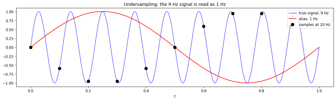
Aliasing happens when the sampling rate is too low for the detail present. A high-frequency sinusoid then becomes indistinguishable from a lower-frequency one: both pass through the same samples. Shannon’s sampling theorem gives the safe rate, \(f_s \ge 2 f_{max}\). Below it, a frequency \(f\) masquerades as the alias \(|f - f_s\,\text{round}(f/f_s)|\). The same effect causes moire on striped shirts, the wagon-wheel illusion in video, and disintegrating checkerboards in graphics.

f, fs = 9, 10                       # 9 Hz sampled at 10 Hz, well below 2*f = 18 Hz
f_alias = abs(f - fs*round(f/fs))   # = 1 Hz

t  = np.linspace(0, 1, 1000)
ts = np.arange(0, 1, 1/fs)
plt.figure(figsize=(13, 4))
plt.plot(t, np.sin(2*np.pi*f*t), 'b', alpha=0.6, label=f'true signal, {f} Hz')
plt.plot(t, np.sin(2*np.pi*f_alias*t), 'r', label=f'alias, {f_alias} Hz')
plt.plot(ts, np.sin(2*np.pi*f*ts), 'ko', ms=8, label=f'samples at {fs} Hz')
plt.legend(loc='upper right'); plt.xlabel('t')
plt.title('Undersampling: the 9 Hz signal is read as 1 Hz')
plt.tight_layout(); plt.show()

print(f'Nyquist needs fs >= 2*f = {2*f} Hz, but fs = {fs} Hz  ->  alias at {f_alias} Hz')

Nyquist needs fs >= 2*f = 18 Hz, but fs = 10 Hz  ->  alias at 1 Hz

4. Aliasing in 2D: moire patterns

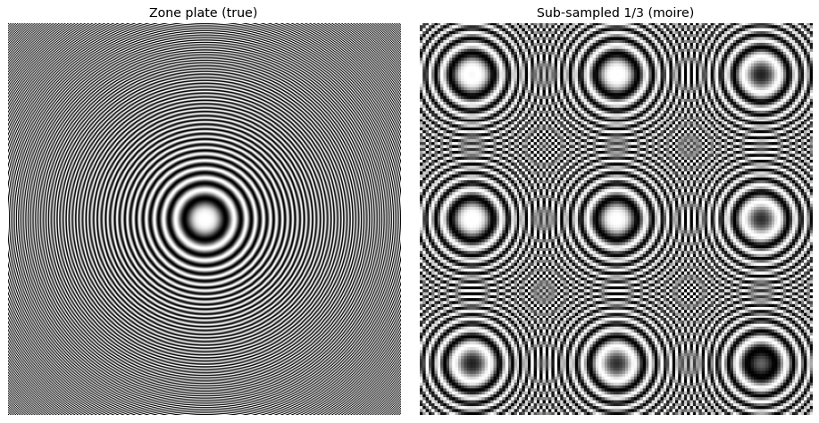
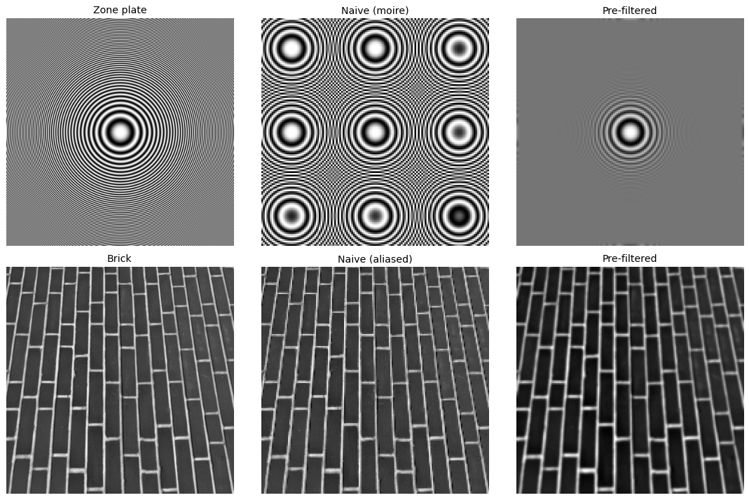
A zone plate, \(\cos(\alpha r^2)\), has a frequency that grows with radius, so its outer rings sit above the Nyquist limit of any coarse grid. Sub-sampling it without care folds those high frequencies back into spurious low-frequency rings: a 2D alias, or moire pattern. The pattern below is entirely an artefact of sampling.

n = 400
y, x = np.mgrid[-n//2:n//2, -n//2:n//2]
zone = 0.5 + 0.5*np.cos((x**2 + y**2) * (np.pi*0.9/n))      # frequency rises with radius
s = 3
naive = resize(zone[::s, ::s], zone.shape, order=0, anti_aliasing=False)   # nearest-upsample to compare

fig, ax = plt.subplots(1, 2, figsize=(11, 5.5))
show(ax[0], zone, 'Zone plate (true)')
show(ax[1], naive, f'Sub-sampled 1/{s} (moire)')
plt.tight_layout(); plt.show()

5. Anti-aliasing by pre-filtering

The fix is to remove the frequencies that cannot be represented before discarding samples. Blurring with a Gaussian (a low-pass filter) first, then sub-sampling, keeps only content the coarse grid can hold, so the moire disappears. This blur-then-sample order is the right way to downscale.

s = 3
def naive_sub(im):  return resize(im[::s, ::s], im.shape, order=0, anti_aliasing=False)
def anti_sub(im):   return resize(ndimage.gaussian_filter(im, 2)[::s, ::s], im.shape, order=0, anti_aliasing=False)

brick = load_gray(data.brick())
fig, ax = plt.subplots(2, 3, figsize=(13, 8.5))
show(ax[0, 0], zone, 'Zone plate');  show(ax[0, 1], naive_sub(zone), 'Naive (moire)');  show(ax[0, 2], anti_sub(zone), 'Pre-filtered')
show(ax[1, 0], brick, 'Brick');      show(ax[1, 1], naive_sub(brick), 'Naive (aliased)'); show(ax[1, 2], anti_sub(brick), 'Pre-filtered')
plt.tight_layout(); plt.show()

6. The Gaussian pyramid

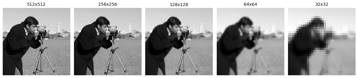
Doing the safe downscale repeatedly, blur then sub-sample by two at each step, builds a Gaussian pyramid: a stack of the same image at halving resolutions. It is a workhorse for multi-scale analysis, coarse-to-fine search, and blending, and is the classical ancestor of the strided downsampling inside convolutional networks.

def gaussian_pyramid(im, levels):
    pyr, cur = [im], im
    for _ in range(levels):
        cur = ndimage.gaussian_filter(cur, 1)[::2, ::2]   # anti-alias, then drop every other sample
        pyr.append(cur)
    return pyr

pyr = gaussian_pyramid(load_gray(data.camera()), 4)
fig, ax = plt.subplots(1, len(pyr), figsize=(14, 4))
for a, level in zip(ax, pyr):
    a.imshow(level, interpolation='nearest'); a.set_title(f'{level.shape[0]}x{level.shape[1]}'); a.axis('off')
plt.tight_layout(); plt.show()

7. Upsampling: interpolation as convolution

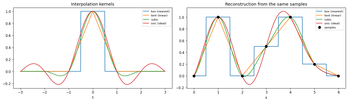
Going the other way, to a higher resolution, we must invent samples between the known ones. Treat the samples as impulses and convolve with an interpolation kernel \(h\):

\[g(i) = \sum_{k} f(k)\, h(i - r k), \qquad r = \text{upsampling rate}\]

The kernel is the method. A box kernel copies the nearest sample (a staircase), a tent gives linear interpolation (piecewise straight), a cubic gives a smooth curve, and the sinc is the ideal band-limited reconstruction, though its slow decay produces ringing near edges.

def k_box(t):   return (np.abs(t) <= 0.5).astype(float)
def k_tent(t):  return np.maximum(0, 1 - np.abs(t))
def k_cubic(t, a=-0.5):
    t = np.abs(t)
    return np.where(t <= 1, (a+2)*t**3 - (a+3)*t**2 + 1,
           np.where(t <  2, a*t**3 - 5*a*t**2 + 8*a*t - 4*a, 0.0))
def k_sinc(t):  return np.sinc(t)            # sin(pi t) / (pi t)

kernels = [('box (nearest)', k_box), ('tent (linear)', k_tent), ('cubic', k_cubic), ('sinc (ideal)', k_sinc)]
samples = np.array([0, 1, 0, 0.5, 1, 0.2, 0], float)

def reconstruct(x, kernel):
    return sum(s*kernel(x - i) for i, s in enumerate(samples))

t  = np.linspace(-3, 3, 600)
xx = np.linspace(0, len(samples)-1, 500)
fig, ax = plt.subplots(1, 2, figsize=(14, 4.2))
for name, ker in kernels:
    ax[0].plot(t, ker(t), label=name)
    ax[1].plot(xx, reconstruct(xx, ker), label=name)
ax[0].set_title('Interpolation kernels'); ax[0].set_xlabel('t'); ax[0].legend(fontsize=8)
ax[1].plot(np.arange(len(samples)), samples, 'ko', ms=7, label='samples')
ax[1].set_title('Reconstruction from the same samples'); ax[1].set_xlabel('x'); ax[1].legend(fontsize=8)
plt.tight_layout(); plt.show()

8. Interpolation in practice: nearest, bilinear, bicubic

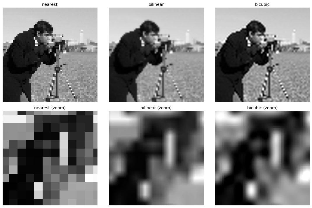
In 2D the same kernels give nearest neighbour (blocky), bilinear (smoother but soft), and bicubic (sharper transitions from the cubic kernel). The zoomed crops make the trade-off visible: higher-order kernels suppress the staircase artefacts at the cost of more computation.

orig  = load_gray(data.camera())
small = orig[::8, ::8]                         # 64 x 64 source to upsample back to 512 x 512
methods = [('nearest', 0), ('bilinear', 1), ('bicubic', 3)]
ups = {name: resize(small, orig.shape, order=o, anti_aliasing=False) for name, o in methods}
cy, cx = 180, 250                              # a crop with fine detail (camera + tripod)

fig, ax = plt.subplots(2, 3, figsize=(13, 8.5))
for j, (name, _) in enumerate(methods):
    show(ax[0, j], ups[name], name)
    ax[1, j].imshow(ups[name][cy:cy+90, cx:cx+90], interpolation='nearest')
    ax[1, j].set_title(f'{name} (zoom)'); ax[1, j].axis('off')
plt.tight_layout(); plt.show()

9. Explore and verify

Two claims here are worth checking numerically: that pre-filtering before sub-sampling really does reduce the error, and that a Gaussian pyramid halves its dimensions at every level. Then we sweep the sampling rate to watch aliasing appear.

# Verify the sampling claims.
from skimage import transform, filters
im = load_gray(data.brick(), size=256)

# 1. Anti-aliased sub-sampling beats naive sub-sampling, measured against a
#    properly band-limited reference.
ref   = transform.resize(im, (128, 128), anti_aliasing=True)
naive = im[::2, ::2]
anti  = filters.gaussian(im, sigma=1.0)[::2, ::2]
e_naive = np.sqrt(np.mean((naive - ref) ** 2))
e_anti  = np.sqrt(np.mean((anti  - ref) ** 2))
assert e_anti < e_naive, 'pre-filtering did not help, which contradicts the lecture'

# 2. Every pyramid level halves the dimensions.
levels = gaussian_pyramid(im, 4)
for i in range(1, len(levels)):
    exp = (levels[i-1].shape[0] + 1) // 2
    assert abs(levels[i].shape[0] - exp) <= 1, f'level {i} is not half of level {i-1}'

print('both checks passed')
print(f'  naive sub-sampling RMSE       = {e_naive:.4f}')
print(f'  pre-filtered sub-sampling RMSE= {e_anti:.4f}   ({e_naive/e_anti:.1f}x better)')
print(f'  pyramid shapes: {[l.shape[0] for l in levels]}')

both checks passed
  naive sub-sampling RMSE       = 0.0411
  pre-filtered sub-sampling RMSE= 0.0288   (1.4x better)
  pyramid shapes: [256, 128, 64, 32, 16]

# Static sweep: sample a fine grating at falling rates and watch aliasing take over.
n = 256
xx = np.arange(n)
fine = 0.5 + 0.5 * np.cos(2 * np.pi * 0.22 * xx)[None, :] * np.ones((n, 1))

fig, ax = plt.subplots(1, 5, figsize=(15, 3.2))
for a, step in zip(ax, [1, 2, 3, 4, 6]):
    sub = fine[::step, ::step]
    a.imshow(sub, cmap='gray'); a.set_axis_off()
    a.set_title(f'every {step}{"st" if step==1 else "th"} pixel\n{sub.shape[0]}x{sub.shape[1]}', fontsize=9)
fig.suptitle('Sub-sampling a 0.22 cycles/pixel grating: past Nyquist the pattern is a lie', y=1.02)
plt.tight_layout(); plt.show()

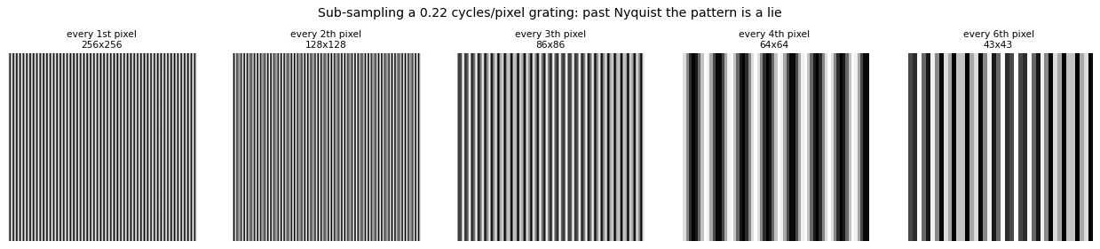
Now the same thing under your control. Drag the slider and watch what changes.

# Live: with and without the anti-aliasing pre-filter, at your chosen rate.
from ipywidgets import interact, IntSlider

def alias(step=4):
    naive = im[::step, ::step]
    anti  = filters.gaussian(im, sigma=0.5 * step)[::step, ::step]
    fig, ax = plt.subplots(1, 2, figsize=(9, 4.4))
    ax[0].imshow(naive, cmap='gray'); ax[0].set_title(f'naive, every {step} px  {naive.shape}')
    ax[1].imshow(anti,  cmap='gray'); ax[1].set_title(f'blur first, then subsample')
    for a in ax: a.set_axis_off()
    plt.tight_layout(); plt.show()

interact(alias, step=IntSlider(min=1, max=8, step=1, value=4, description='keep every'));

---

Key takeaways

Concept	Key takeaway
Convolution cost	Spatial is \(O(N^2 k^2)\); the FFT route is about \(O(N^2 \log N^2)\) and wins for large kernels
Sub-sampling	Dropping rows and columns discards high frequencies carelessly and looks broken
Aliasing	When \(f_s < 2 f_{max}\) a high frequency masquerades as a lower one (moire, wagon-wheel)
Nyquist rate	Sample at \(f_s \ge 2 f_{max}\) to represent a band-limited signal faithfully
Anti-aliasing	Low-pass (blur) before sub-sampling, so only representable content remains
Gaussian pyramid	Repeated blur-then-subsample-by-2; a multi-scale stack for coarse-to-fine vision
Interpolation	Upsampling convolves samples with a kernel \(h\): \(g(i)=\sum_k f(k)\,h(i-rk)\)
Kernels	Box gives nearest, tent gives linear, cubic gives smooth, sinc is ideal but rings
Decimation	Downsampling is also a convolution: \(g(i)=\sum_k f(k)\,h(i-k/r)\)

Reading: Szeliski, Computer Vision: Algorithms and Applications, Ch. 3 (3.5.1-3.5.2); Forsyth and Ponce, Computer Vision: A Modern Approach, Ch. 7 (7.4).

References: S. Seitz; R. Urtasun (Toronto); N. Snavely (Cornell); B. Curless (UW).

Exercises

1. Find the Nyquist rate empirically. Sample \(\sin(2\pi f t)\) at decreasing rates and find the smallest \(f_s\) that still reconstructs the signal. Check it against \(f_s \ge 2f_{max}\).

2. Anti-aliasing, measured. Sub-sample a checkerboard with and without a pre-blur. Compare both against a properly filtered reference and report the error numerically, not just visually.

3. Gaussian pyramid round trip. Build a pyramid, confirm each level halves the dimensions, then reconstruct upward and measure what was lost. Why is this loss not recoverable?

4. Interpolation trade-offs. Upsample a small image with nearest, bilinear and bicubic. Rank them for blockiness, blur and ringing, and say which you would use for a photograph versus a segmentation mask.