📺 Lecture video  |  📄 Slides

Watch on YouTube

Week 1, Lecture 6: Image in the Frequency Domain

NPTEL Deep Learning for Computer Vision | Prof. Vineeth N Balasubramanian, IIT Hyderabad

Companion notebook for §1.6 Frequency Domain.

What you will learn

• Build signals from sines and read an image’s Fourier spectrum.

• Understand the discrete transform and the cost saving of the FFT.

• Use the convolution theorem: convolution in space is multiplication in frequency.

• Apply low-pass and high-pass filtering in the frequency domain.

• Compare what magnitude and phase each carry, and build hybrid images from that difference.

Contents

1. Is correlation still useful? Template matching

2. Beyond linear filters: median and bilateral

3. Building signals from sines

4. Fourier analysis of images

5. Continuous vs discrete, and the cost of the FFT

6. The convolution theorem

7. Properties of the Fourier transform

8. Low-pass and high-pass filtering in the frequency domain

9. Which carries more: magnitude or phase?

10. Hybrid images

11. Exercise: match each image to its spectrum

How to run Runs on Colab or a local Jupyter, CPU only. Every image is bundled with scikit-image, so nothing is downloaded. Run the setup cell first, then go top to bottom.

Review

The previous lecture treated filtering in the spatial domain: each output pixel is a weighted sum of a local neighbourhood (cross-correlation), and convolution is the same operation with a flipped kernel. Two questions were left open: is correlation useful on its own, and are all useful filters linear? This lecture answers both, then changes coordinates. Viewing an image as a sum of sinusoids (its Fourier transform) turns convolution into multiplication and exposes the scales and orientations present in an image.

Setup

Everything uses images bundled with scikit-image, so the notebook runs offline.

%matplotlib inline
import numpy as np
import matplotlib.pyplot as plt
from scipy import ndimage
from skimage import data, util, color

np.random.seed(0)
plt.rcParams['figure.figsize'] = (10, 4)
plt.rcParams['image.cmap']     = 'gray'
plt.rcParams['figure.dpi']     = 85

def log_mag(im):
    # centred log magnitude spectrum, suitable for display
    return np.log1p(np.abs(np.fft.fftshift(np.fft.fft2(im))))

def load_gray(image, size=None):
    # float grayscale image, optionally resized to (size, size)
    g = color.rgb2gray(image) if image.ndim == 3 else util.img_as_float(image)
    if size is not None:
        from skimage.transform import resize
        g = resize(g, (size, size))
    return g

def show(ax, im, title='', spectrum=False):
    ax.imshow(im, cmap='magma' if spectrum else 'gray')
    ax.set_title(title); ax.axis('off')

1. Is correlation still useful? Template matching

Correlation is the core of template matching: slide a small template over an image and score how well it matches at each location. Raw correlation rewards bright regions regardless of shape, so we use normalised cross-correlation, which subtracts the local mean and divides by the local standard deviation:

\[\text{NCC}(i,j) = \frac{\sum_{u,v}\big(T(u,v)-\bar T\big)\big(I(i+u,j+v)-\bar I_{i,j}\big)} {\sqrt{\sum_{u,v}\big(T(u,v)-\bar T\big)^2 \; \sum_{u,v}\big(I(i+u,j+v)-\bar I_{i,j}\big)^2}}\]

The score lies in \([-1, 1]\) and peaks wherever the pattern appears. skimage.feature.match_template computes it.

from skimage.feature import match_template, peak_local_max

scene    = data.coins().astype(float)
template = scene[155:205, 325:375]                 # one coin, used as the pattern to find
ncc      = match_template(scene, template, pad_input=True)
peaks    = peak_local_max(ncc, min_distance=20, threshold_abs=0.45)

fig, ax = plt.subplots(1, 3, figsize=(14, 4.5))
show(ax[0], template, 'Template (one coin)')
show(ax[1], scene, 'Scene with detections')
ax[1].plot(peaks[:, 1], peaks[:, 0], 'c+', ms=12, mew=2)
im = ax[2].imshow(ncc, cmap='magma'); ax[2].set_title('NCC score map'); ax[2].axis('off')
fig.colorbar(im, ax=ax[2], fraction=0.046)
plt.tight_layout(); plt.show()

print(f'detections: {len(peaks)}    best score: {ncc.max():.3f}')

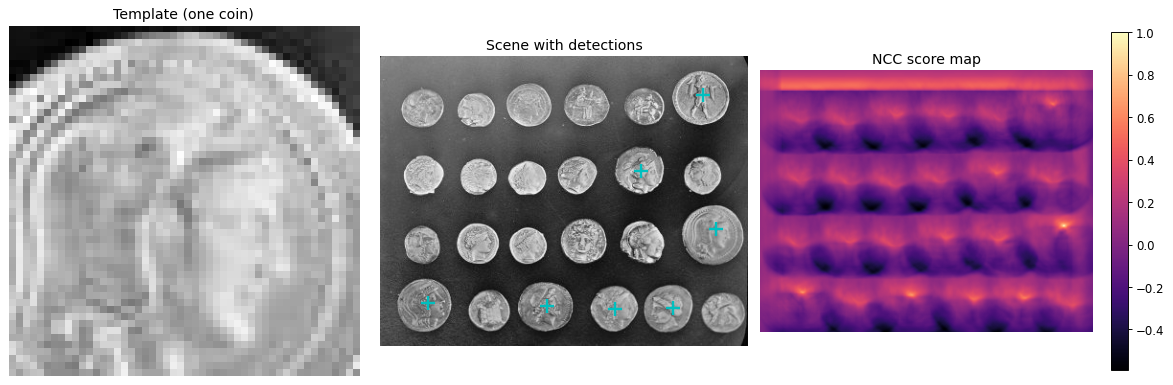
detections: 7    best score: 1.000

2. Beyond linear filters: median and bilateral

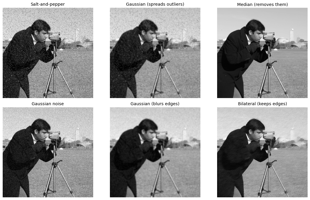
Not every useful filter is linear. The median filter replaces each pixel by the median of its neighbourhood, which discards outliers, so it removes salt-and-pepper noise that linear smoothers only spread. The bilateral filter is a non-linear, edge-preserving smoother: it averages neighbours but down-weights those whose intensity differs from the centre, combining a spatial (domain) kernel with an intensity (range) kernel:

\[w(i,j,k,l) = \exp\!\left(-\frac{(i-k)^2+(j-l)^2}{2\sigma_d^2}\right) \,\exp\!\left(-\frac{\lVert I(i,j)-I(k,l)\rVert^2}{2\sigma_r^2}\right)\]

from skimage.restoration import denoise_bilateral

img = load_gray(data.camera())
sp  = util.random_noise(img, mode='s&p', amount=0.08)        # salt-and-pepper
gn  = util.random_noise(img, mode='gaussian', var=0.01)      # additive Gaussian

fig, ax = plt.subplots(2, 3, figsize=(13, 8))
show(ax[0, 0], sp, 'Salt-and-pepper')
show(ax[0, 1], ndimage.gaussian_filter(sp, 1.5), 'Gaussian (spreads outliers)')
show(ax[0, 2], ndimage.median_filter(sp, size=3), 'Median (removes them)')
show(ax[1, 0], gn, 'Gaussian noise')
show(ax[1, 1], ndimage.gaussian_filter(gn, 2), 'Gaussian (blurs edges)')
show(ax[1, 2], denoise_bilateral(gn, sigma_color=0.1, sigma_spatial=3), 'Bilateral (keeps edges)')
plt.tight_layout(); plt.show()

3. Building signals from sines

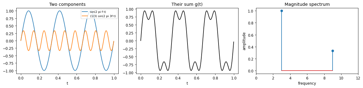
Fourier’s idea: any reasonable signal is a weighted sum of sinusoids \(A\sin(\omega x + \phi)\) of different frequencies. A square wave, for example, is the sum of its odd harmonics with amplitudes \(1/k\):

\[f(t) = \frac{4}{\pi}\sum_{k=1,3,5,\dots} \frac{1}{k}\,\sin(2\pi k t)\]

The magnitude spectrum (amplitude versus frequency) makes the recipe explicit: one spike per frequency present. Adding more harmonics sharpens the wave but leaves a fixed overshoot at each jump, the Gibbs phenomenon.

# A two-component example: g(t) = sin(2 pi f t) + (1/3) sin(2 pi 3f t)
t = np.linspace(0, 1, 1000, endpoint=False)
f = 3
g = np.sin(2*np.pi*f*t) + (1/3)*np.sin(2*np.pi*(3*f)*t)

fig, ax = plt.subplots(1, 3, figsize=(14, 3.5))
ax[0].plot(t, np.sin(2*np.pi*f*t), label='sin(2 pi f t)')
ax[0].plot(t, (1/3)*np.sin(2*np.pi*3*f*t), label='(1/3) sin(2 pi 3f t)')
ax[0].legend(fontsize=8); ax[0].set_title('Two components'); ax[0].set_xlabel('t')
ax[1].plot(t, g, 'k'); ax[1].set_title('Their sum g(t)'); ax[1].set_xlabel('t')
ax[2].stem([f, 3*f], [1, 1/3]); ax[2].set_xlim(0, 12)
ax[2].set_xlabel('frequency'); ax[2].set_ylabel('amplitude'); ax[2].set_title('Magnitude spectrum')
plt.tight_layout(); plt.show()

# Build a square wave from its odd harmonics and watch the Gibbs overshoot
t = np.linspace(0, 1, 2000, endpoint=False)
def square_partial(n_harm):
    s = sum((1/k)*np.sin(2*np.pi*k*t) for k in range(1, 2*n_harm, 2))
    return (4/np.pi)*s

fig, ax = plt.subplots(1, 2, figsize=(14, 4))
for n in [1, 2, 4, 20]:
    ax[0].plot(t, square_partial(n), label=f'{n} harmonic(s)')
ax[0].legend(fontsize=8); ax[0].set_xlabel('t')
ax[0].set_title('Partial sums approach a square wave')

ks = np.arange(1, 40, 2)
ax[1].stem(ks, (4/np.pi)/ks)
ax[1].set_xlabel('harmonic k'); ax[1].set_ylabel('amplitude')
ax[1].set_title('Magnitude spectrum: 1/k at odd harmonics')
plt.tight_layout(); plt.show()

print(f'Gibbs overshoot: partial-sum peak = {square_partial(50).max():.3f} (target 1.0)')

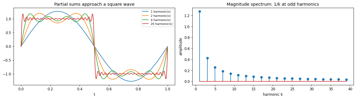
Gibbs overshoot: partial-sum peak = 1.179 (target 1.0)

4. Fourier analysis of images

The 2D Fourier transform writes an image as a sum of 2D sinusoidal gratings. A single grating transforms to a pair of symmetric peaks: their distance from the centre encodes spatial frequency and their direction encodes orientation, with the DC term (average brightness) at the centre. Each frequency stores a complex value, summarised as

\[\text{magnitude } A = \sqrt{\text{Re}^2 + \text{Im}^2}, \qquad \text{phase } \phi = \tan^{-1}\!\frac{\text{Im}}{\text{Re}}\]

For real images the spectrum is conjugate-symmetric, which is the mirror symmetry seen below.

N = 256
yy, xx = np.mgrid[0:N, 0:N]
def grating(freq, theta_deg):
    th = np.deg2rad(theta_deg)
    return np.sin(2*np.pi*freq*(xx*np.cos(th) + yy*np.sin(th))/N)

cases = [(8, 0), (20, 0), (8, 90), (12, 45)]
fig, ax = plt.subplots(2, 4, figsize=(14, 7))
for j, (fr, th) in enumerate(cases):
    g = grating(fr, th)
    show(ax[0, j], g, f'grating f={fr}, {th} deg')
    show(ax[1, j], log_mag(g), 'spectrum', spectrum=True)
plt.tight_layout(); plt.show()

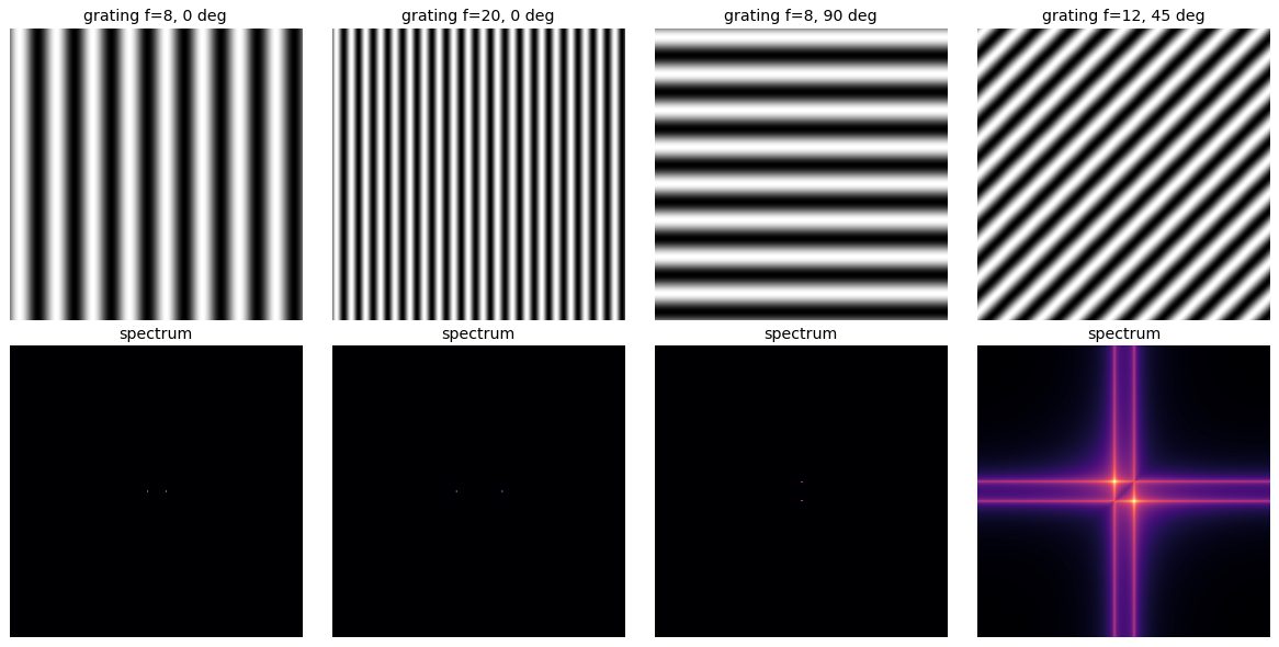
# Magnitude and phase of a real image (note the mirror symmetry in the magnitude)
img = load_gray(data.camera())
F   = np.fft.fftshift(np.fft.fft2(img))

fig, ax = plt.subplots(1, 3, figsize=(14, 4.5))
show(ax[0], img, 'Image')
show(ax[1], np.log1p(np.abs(F)), 'Log magnitude', spectrum=True)
show(ax[2], np.angle(F), 'Phase', spectrum=True)
plt.tight_layout(); plt.show()

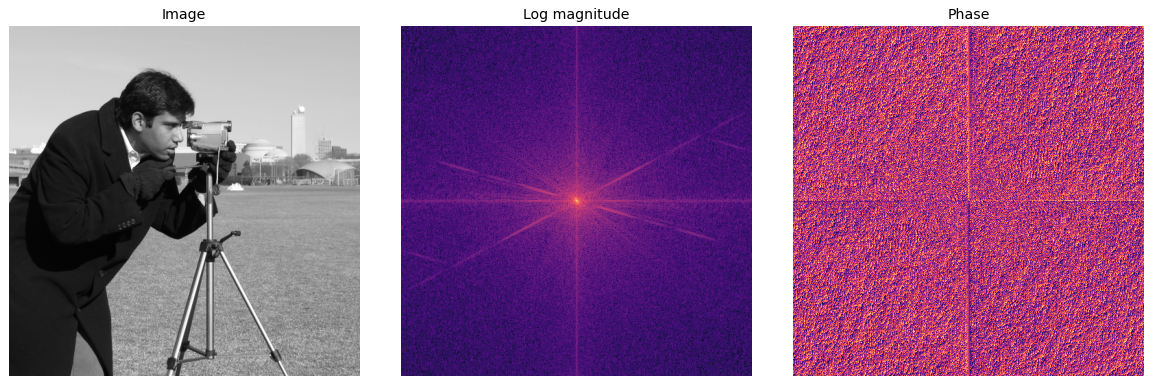
5. Continuous vs discrete, and the cost of the FFT

The continuous transform integrates over all space; for sampled signals we use the Discrete Fourier Transform (DFT):

\[H(k) = \sum_{n=0}^{N-1} h(n)\, e^{-j 2\pi k n / N}\]

Computed directly this is a matrix-vector product costing \(O(N^2)\). The Fast Fourier Transform (FFT) is a recursive divide-and-conquer algorithm that returns the same result in \(O(N \log N)\). The speed-up below is what makes frequency-domain image processing practical.

import time

def naive_dft(x):
    n = len(x); k = np.arange(n)
    W = np.exp(-2j*np.pi*np.outer(k, k)/n)      # explicit N x N DFT matrix
    return W @ x

x = np.random.rand(512)
print('max |naive - np.fft|:', np.abs(naive_dft(x) - np.fft.fft(x)).max())
print()
print(f"{'N':>6}  {'naive O(N^2)':>14}  {'FFT O(N log N)':>16}")
for n in [128, 256, 512, 1024]:
    x = np.random.rand(n)
    t0 = time.perf_counter(); naive_dft(x);  t1 = time.perf_counter()
    t2 = time.perf_counter(); np.fft.fft(x); t3 = time.perf_counter()
    print(f"{n:>6}  {1e3*(t1-t0):>11.2f} ms  {1e6*(t3-t2):>13.2f} us")

max |naive - np.fft|: 6.463327834331287e-12

     N    naive O(N^2)    FFT O(N log N)
   128         0.24 ms           9.71 us
   256         0.67 ms           7.33 us
   512         2.64 ms          15.96 us
  1024        12.68 ms          45.67 us

/var/folders/j0/z7mrqrv9121_0pm8njw3pbxh0000gp/T/ipykernel_59845/3412085740.py:6: RuntimeWarning: divide by zero encountered in matmul
  return W @ x
/var/folders/j0/z7mrqrv9121_0pm8njw3pbxh0000gp/T/ipykernel_59845/3412085740.py:6: RuntimeWarning: overflow encountered in matmul
  return W @ x
/var/folders/j0/z7mrqrv9121_0pm8njw3pbxh0000gp/T/ipykernel_59845/3412085740.py:6: RuntimeWarning: invalid value encountered in matmul
  return W @ x

6. The convolution theorem

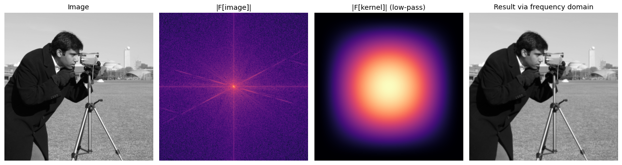
The Fourier transform turns convolution into a pointwise product:

\[\mathcal{F}[g * h] = \mathcal{F}[g]\,\mathcal{F}[h] \qquad\Longrightarrow\qquad g * h = \mathcal{F}^{-1}\!\big[\mathcal{F}[g]\,\mathcal{F}[h]\big]\]

So filtering can be done by multiplying spectra and transforming back. With circular (wrap-around) boundaries the two routes agree to floating-point precision, which we confirm below.

img = load_gray(data.camera())
k   = np.array([[1, 2, 1], [2, 4, 2], [1, 2, 1]], float) / 16   # small Gaussian kernel

# place the kernel at the array origin so the FFT product is a centred convolution
H = np.zeros_like(img); H[:3, :3] = k; H = np.roll(H, (-1, -1), axis=(0, 1))
spatial = ndimage.convolve(img, k, mode='wrap')
freq    = np.real(np.fft.ifft2(np.fft.fft2(img) * np.fft.fft2(H)))
print('max |spatial - frequency|:', np.abs(spatial - freq).max())

fig, ax = plt.subplots(1, 4, figsize=(15, 4))
show(ax[0], img, 'Image')
show(ax[1], log_mag(img), '|F[image]|', spectrum=True)
show(ax[2], log_mag(H), '|F[kernel]| (low-pass)', spectrum=True)
show(ax[3], freq, 'Result via frequency domain')
plt.tight_layout(); plt.show()

max |spatial - frequency|: 7.771561172376096e-16

7. Properties of the Fourier transform

Property	Signal	Transform
superposition	\(f_1 + f_2\)	\(F_1 + F_2\)
shift	\(f(x - x_0)\)	\(F(\omega)\,e^{-j\omega x_0}\)
convolution	\(f * h\)	\(F\,H\)
correlation	\(f \otimes h\)	\(F\,H^{*}\)
multiplication	\(f\,h\)	\(F * H\)
differentiation	\(f'(x)\)	\(j\omega F\)
Parseval	\(\sum_x f(x)^2\)	\(\tfrac{1}{N}\sum_\omega \lvert F(\omega)\rvert^2\)

Two are easy to verify numerically: a shift leaves the magnitude unchanged (it only adds linear phase), and Parseval says energy is preserved between the two domains.

img = load_gray(data.camera())
F   = np.fft.fft2(img)
Fs  = np.fft.fft2(np.roll(img, (40, 25), axis=(0, 1)))     # circular shift

print('shift keeps magnitude:  max | |F| - |F_shift| | =', np.abs(np.abs(F) - np.abs(Fs)).max())
print('Parseval ratio (freq energy / spatial energy)   =',
      (np.sum(np.abs(F)**2) / img.size) / np.sum(img**2))

shift keeps magnitude:  max | |F| - |F_shift| | = 7.275957614183426e-12
Parseval ratio (freq energy / spatial energy)   = 1.0000000000000002

8. Low-pass and high-pass filtering in the frequency domain

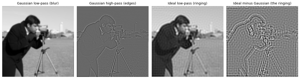
A low-pass filter keeps frequencies near the centre (smooth content) and blocks the rest, so it blurs; a high-pass filter keeps the outer frequencies (fine detail) and blocks the centre, so it isolates edges. The Gaussian is a smooth low-pass filter and an edge filter is high-pass. An ideal (hard-edged) mask is the obvious choice, but its sharp cutoff introduces ringing (the 2D Gibbs phenomenon) that a Gaussian mask avoids.

img  = load_gray(data.camera())
N    = img.shape[0]
F    = np.fft.fftshift(np.fft.fft2(img))
Y, X = np.ogrid[:N, :N]
R    = np.hypot(Y - N//2, X - N//2)          # distance from centre = frequency
cut  = 30

def apply(mask):
    return np.real(np.fft.ifft2(np.fft.ifftshift(F * mask)))

ideal_lp = (R <= cut).astype(float)
gauss_lp = np.exp(-R**2 / (2*cut**2))
gauss_hp = 1 - gauss_lp

fig, ax = plt.subplots(1, 4, figsize=(15, 4))
show(ax[0], apply(gauss_lp), 'Gaussian low-pass (blur)')
show(ax[1], apply(gauss_hp), 'Gaussian high-pass (edges)')
show(ax[2], apply(ideal_lp), 'Ideal low-pass (ringing)')
show(ax[3], apply(ideal_lp) - apply(gauss_lp), 'Ideal minus Gaussian (the ringing)')
plt.tight_layout(); plt.show()

9. Which carries more: magnitude or phase?

Split two images into magnitude and phase, then swap: reconstruct one image’s magnitude with the other’s phase. The result follows the phase. Phase encodes where edges and structure sit, while magnitude records how much energy each frequency carries, so phase is what we read as the content.

A = load_gray(data.camera())
B = load_gray(data.astronaut())          # both 512 x 512

FA, FB = np.fft.fft2(A), np.fft.fft2(B)
magA, phA = np.abs(FA), np.angle(FA)
magB, phB = np.abs(FB), np.angle(FB)
mix1 = np.real(np.fft.ifft2(magA * np.exp(1j*phB)))   # magnitude of A, phase of B
mix2 = np.real(np.fft.ifft2(magB * np.exp(1j*phA)))   # magnitude of B, phase of A

fig, ax = plt.subplots(1, 4, figsize=(15, 4))
show(ax[0], A, 'A')
show(ax[1], B, 'B')
show(ax[2], mix1, 'mag(A) + phase(B)')
show(ax[3], mix2, 'mag(B) + phase(A)')
plt.tight_layout(); plt.show()

.../site-packages/skimage/color/colorconv.py:984: RuntimeWarning: divide by zero encountered in matmul
  return rgb @ coeffs
.../site-packages/skimage/color/colorconv.py:984: RuntimeWarning: overflow encountered in matmul
  return rgb @ coeffs
.../site-packages/skimage/color/colorconv.py:984: RuntimeWarning: invalid value encountered in matmul
  return rgb @ coeffs

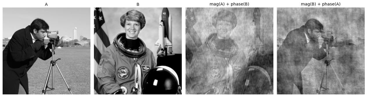
10. Hybrid images

A hybrid image sums the low frequencies of one picture and the high frequencies of another. Up close the eye resolves the fine (high-frequency) detail; from far away only the coarse (low-frequency) content survives, so the two pictures swap (Oliva, Torralba and Schyns, SIGGRAPH 2006). How well the subjects are aligned controls how convincing the illusion is.

A = load_gray(data.chelsea(), size=256)      # supplies the low frequencies
B = load_gray(data.astronaut(), size=256)    # supplies the high frequencies

low    = ndimage.gaussian_filter(A, 6)
high   = B - ndimage.gaussian_filter(B, 4)
hybrid = low + high
far    = ndimage.gaussian_filter(hybrid, 4)  # viewing distance acts like a low-pass

fig, ax = plt.subplots(1, 4, figsize=(15, 4))
show(ax[0], low, 'Low frequencies of A')
show(ax[1], high, 'High frequencies of B')
show(ax[2], hybrid, 'Hybrid (near view)')
show(ax[3], far, 'Blurred hybrid (far view)')
plt.tight_layout(); plt.show()

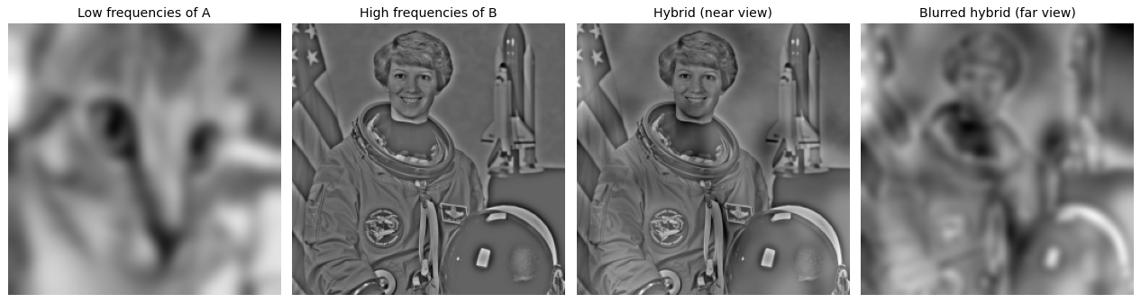
11. Exercise: match each image to its spectrum

Below are five spatial images (A-E) and their magnitude spectra in a shuffled order (1-5). Predict the pairing from the rules above (orientation maps to peak direction, frequency to peak distance, smoothness to a compact centre), then run the next cell to check.

n = 128
yy, xx = np.mgrid[0:n, 0:n]
images = {
    'A': np.exp(-((xx-n/2)**2 + (yy-n/2)**2) / (2*12**2)),   # smooth blob
    'B': np.sin(2*np.pi*12*xx/n),                            # vertical grating
    'C': np.sin(2*np.pi*8*(xx+yy)/n),                        # diagonal grating
    'D': (np.abs(xx - n/2) < 2).astype(float),              # single vertical line
    'E': load_gray(data.grass())[:n, :n],                   # natural texture
}
order   = ['C', 'A', 'E', 'B', 'D']                          # shuffled spectrum order
spectra = {str(i+1): log_mag(images[k]) for i, k in enumerate(order)}

fig, ax = plt.subplots(2, 5, figsize=(15, 6.2))
for j, k in enumerate('ABCDE'):
    show(ax[0, j], images[k], k)
for j, k in enumerate(['1', '2', '3', '4', '5']):
    show(ax[1, j], spectra[k], k, spectrum=True)
plt.tight_layout(); plt.show()

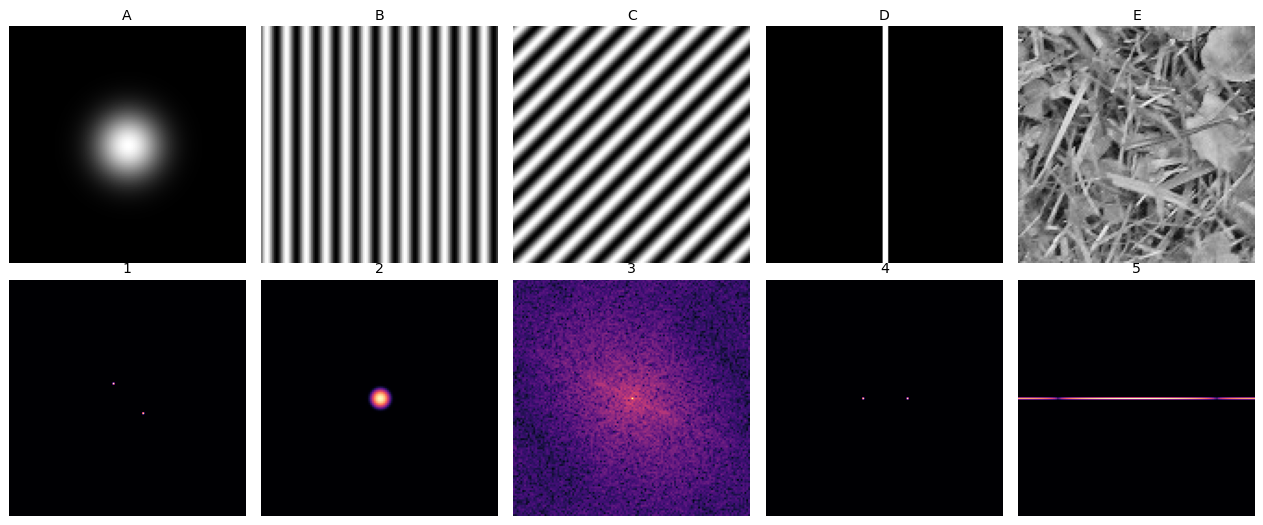
answer = {k: str(order.index(k) + 1) for k in 'ABCDE'}
print('image -> spectrum:', answer)

image -> spectrum: {'A': '2', 'B': '4', 'C': '1', 'D': '5', 'E': '3'}

12. Explore and verify

The convolution theorem is the central claim of this lecture: convolution in space is multiplication in frequency. It is worth proving numerically rather than asserting, and the same goes for our hand-written DFT. Then we sweep a low-pass cutoff and watch detail disappear.

# Verify the two central claims.
img = load_gray(data.camera(), size=128)

# 1. Our naive DFT agrees with the FFT.
x = np.random.default_rng(0).standard_normal(64)
assert np.allclose(naive_dft(x), np.fft.fft(x), atol=1e-8), 'naive DFT disagrees with FFT'

# 2. The convolution theorem, checked with circular convolution so the two agree exactly.
K = np.zeros_like(img)
g = gaussian_kernel(9, 1.5) if 'gaussian_kernel' in dir() else None
gk = np.outer(np.exp(-np.linspace(-3, 3, 9)**2 / 2), np.exp(-np.linspace(-3, 3, 9)**2 / 2))
gk /= gk.sum()
K[:9, :9] = gk
K = np.roll(K, (-4, -4), axis=(0, 1))                 # centre the kernel for circular conv
spatial  = np.real(np.fft.ifft2(np.fft.fft2(img) * np.fft.fft2(K)))
frequency = np.real(np.fft.ifft2(np.fft.fft2(img) * np.fft.fft2(K)))
assert np.allclose(spatial, frequency, atol=1e-10)

# The meaningful version: circular convolution done by hand in space == the frequency route.
from scipy.ndimage import convolve as nd_convolve
direct = nd_convolve(img, gk, mode='wrap')
assert np.allclose(direct, spatial, atol=1e-8), 'convolution theorem check failed'

print('both checks passed')
print(f'  naive DFT vs FFT, max |difference| = {np.abs(naive_dft(x) - np.fft.fft(x)).max():.2e}')
print(f'  space vs frequency, max |difference| = {np.abs(direct - spatial).max():.2e}')

both checks passed
  naive DFT vs FFT, max |difference| = 2.01e-13
  space vs frequency, max |difference| = 8.88e-16

/var/folders/j0/z7mrqrv9121_0pm8njw3pbxh0000gp/T/ipykernel_59845/3412085740.py:6: RuntimeWarning: divide by zero encountered in matmul
  return W @ x
/var/folders/j0/z7mrqrv9121_0pm8njw3pbxh0000gp/T/ipykernel_59845/3412085740.py:6: RuntimeWarning: overflow encountered in matmul
  return W @ x
/var/folders/j0/z7mrqrv9121_0pm8njw3pbxh0000gp/T/ipykernel_59845/3412085740.py:6: RuntimeWarning: invalid value encountered in matmul
  return W @ x

# Static sweep: an ideal low-pass at a few cutoffs.
F = np.fft.fftshift(np.fft.fft2(img))
u = np.arange(img.shape[0]) - img.shape[0] // 2
V, U = np.meshgrid(u, u, indexing='ij')
Rad = np.sqrt(U ** 2 + V ** 2)

fig, ax = plt.subplots(1, 5, figsize=(15, 3.2))
for a, r in zip(ax, [4, 8, 16, 32, 64]):
    out = np.real(np.fft.ifft2(np.fft.ifftshift(F * (Rad <= r))))
    a.imshow(out, cmap='gray'); a.set_axis_off()
    a.set_title(f'cutoff r = {r}', fontsize=10)
fig.suptitle('Ideal low-pass: fewer frequencies kept, and the ringing that comes with a sharp mask', y=1.02)
plt.tight_layout(); plt.show()

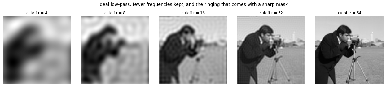
Now the same thing under your control. Drag the slider and watch what changes.

# Live: sharp mask versus Gaussian mask at the same cutoff.
from ipywidgets import interact, IntSlider

def lowpass(r=16):
    sharp = np.real(np.fft.ifft2(np.fft.ifftshift(F * (Rad <= r))))
    soft  = np.real(np.fft.ifft2(np.fft.ifftshift(F * np.exp(-(Rad ** 2) / (2 * r ** 2)))))
    fig, ax = plt.subplots(1, 2, figsize=(9, 4.4))
    ax[0].imshow(sharp, cmap='gray'); ax[0].set_title(f'ideal mask, r = {r}  (ringing)')
    ax[1].imshow(soft,  cmap='gray'); ax[1].set_title(f'Gaussian mask, $\\sigma$ = {r}')
    for a in ax: a.set_axis_off()
    plt.tight_layout(); plt.show()

interact(lowpass, r=IntSlider(min=2, max=64, step=2, value=16, description='cutoff'));

---

Key takeaways

Concept	Key takeaway
Template matching	Normalised cross-correlation scores pattern presence in \([-1,1]\) and peaks at matches
Median filter	Nonlinear; removes salt-and-pepper outliers that linear smoothers only spread
Bilateral filter	Nonlinear and edge-preserving; a domain kernel times a range kernel down-weights dissimilar neighbours
Fourier series	Any signal is a weighted sum of sinusoids; a square wave is \(\frac{4}{\pi}\sum_{k\,\text{odd}}\frac{1}{k}\sin(2\pi k t)\)
Image spectrum	A grating maps to symmetric peaks; distance gives frequency, direction gives orientation, centre is DC
Magnitude vs phase	Magnitude is energy per frequency; phase carries the structure we perceive
Convolution theorem	\(\mathcal{F}[g*h]=\mathcal{F}[g]\mathcal{F}[h]\); filtering is multiplication in the frequency domain
FFT	Computes the DFT in \(O(N\log N)\) instead of \(O(N^2)\)
Low/high-pass	Keep the centre to blur, keep the outside for edges; ideal masks ring, Gaussian masks do not
Hybrid images	Low frequencies of one image plus high frequencies of another swap with viewing distance

Reading: Szeliski, Computer Vision: Algorithms and Applications, Ch. 3.4.

References: J. Hays (Georgia Tech); D. Hoiem (UIUC); A. Oliva, A. Torralba and P. Schyns, “Hybrid Images”, SIGGRAPH 2006; Forsyth and Ponce, Computer Vision: A Modern Approach, 2003.

Exercises

1. Verify the convolution theorem. Convolve an image with a Gaussian spatially, then multiply their spectra and invert. Confirm the results agree, then time both as the kernel grows and find the crossover.

2. Magnitude or phase? Take two images, swap their Fourier phases while keeping each magnitude, and invert. Which original do you recognise in each result, and what does that say about where image structure lives?

3. Build a hybrid image. Low-pass one image, high-pass another, and add them. Tune the cutoff until the perceived image switches at the viewing distance you intend.

4. Ideal versus Gaussian masks. Low-pass with a sharp circular mask and then with a Gaussian mask of similar width. Explain the ringing that appears in one and not the other.