Week 5, Lecture 3: Finetuning CNNs (Transfer Learning)

Week 5, Lecture 3: Finetuning CNNs (Transfer Learning)#

NPTEL Deep Learning for Computer Vision | Prof. Vineeth N Balasubramanian, IIT Hyderabad

Companion notebook for §5.3 Finetuning in CNNs.

Training a deep CNN from scratch needs lots of data, compute, and careful tuning. This lecture shows how to instead reuse a network pretrained on a large dataset (ImageNet) and adapt it to a new task with very little data. This is transfer learning, the workhorse of practical computer vision.

What you will learn

Understand why training CNNs from scratch is hard: optimization, overfitting, and compute cost.
See that CNN features are hierarchical: early layers are generic (edges, colors), later layers are specialized.
Understand transfer learning and its two modes: feature extraction vs fine-tuning.
Freeze and unfreeze layers in PyTorch and count trainable parameters.
Run a hands-on transfer-learning micro-demo on a tiny dataset and beat a from-scratch baseline.
Choose the right strategy based on dataset size and domain similarity.

Contents

Why finetune? Training from scratch is hard
Hierarchical features: generic early, specialized late
The transfer learning idea
Freezing layers in PyTorch
Hands-on micro-demo: feature extraction on a tiny CIFAR-10 subset
Decision guide: which strategy to use
Fine-tuning tips

How to run

Self-contained: every import and download happens inside the notebook.
Runs on CPU or GPU, locally or on Google Colab. All cells are kept tiny and fast.
Interactive: several cells build a widget. Run the cell, then drag the slider or pick from the dropdown and watch the output update.
Reproducible: seeds are set in the setup cell below.

Review#

The previous lecture surveyed the modern architectures, from WideResNet and ResNeXt through DenseNet, MobileNet and ConvNeXt. Every one of them assumes you can train from scratch on a large dataset. This lecture covers what to do when you cannot.

Setup#

# Setup: runs on CPU or GPU, on Colab or locally.
import sys, math, time
import numpy as np
import torch
import torch.nn as nn
import torch.nn.functional as F
import matplotlib.pyplot as plt

# ipywidgets is preinstalled on Colab; install only if missing.
try:
    import ipywidgets as widgets
    from ipywidgets import interact, interactive
except ImportError:
    import subprocess
    subprocess.run([sys.executable, "-m", "pip", "install", "-q", "ipywidgets"])
    import ipywidgets as widgets
    from ipywidgets import interact, interactive

torch.manual_seed(0)
np.random.seed(0)
device = torch.device('cuda' if torch.cuda.is_available() else 'cpu')
print('Using device:', device)

def count_params(module):
    """Total number of parameters in a module."""
    return sum(p.numel() for p in module.parameters())

def count_trainable(module):
    """Number of parameters that will receive gradients."""
    return sum(p.numel() for p in module.parameters() if p.requires_grad)

plt.rcParams['figure.dpi'] = 110
plt.rcParams['font.size'] = 10

Using device: cpu

1. Why finetune? Training from scratch is hard#

Training a deep CNN from random initialization is expensive on three axes:

Optimization is delicate. Deep nets need careful weight initialization, normalization, and learning-rate schedules to converge at all.
Overfitting on small data. A network with tens of millions of parameters memorizes a small dataset instead of generalizing.
Compute is heavy. The classic ImageNet models took days to weeks on multiple GPUs to train.

Parameter counts and original training cost (approximate):

Model	Parameters	Original training time
AlexNet	~60M	5 to 6 days
VGG-16	~138M	2 to 3 weeks
Inception-v1 (GoogLeNet)	~5M	~1 week
ResNet-50	~25M	(days on multiple GPUs)

Takeaway: if someone already paid this cost on ImageNet, we should reuse their trained weights rather than start over.

# Sanity check: count parameters of standard torchvision models (structure only, no weights).
import torchvision.models as models

specs = [
    ("AlexNet",      models.alexnet(weights=None),      "5 to 6 days"),
    ("VGG-16",       models.vgg16(weights=None),        "2 to 3 weeks"),
    ("Inception-v1", models.googlenet(weights=None, init_weights=False), "~1 week"),
    ("ResNet-50",    models.resnet50(weights=None),     "days, multi-GPU"),
]

print(f"{'Model':<14}{'Params (M)':>12}   {'Train time':<16}")
print("-" * 46)
for name, m, t in specs:
    p = count_params(m) / 1e6
    print(f"{name:<14}{p:>12.1f}   {t:<16}")
print("\nHuge param counts + long training = strong reason to reuse pretrained weights.")

Model           Params (M)   Train time      
----------------------------------------------
AlexNet               61.1   5 to 6 days     
VGG-16               138.4   2 to 3 weeks    
Inception-v1          13.0   ~1 week         
ResNet-50             25.6   days, multi-GPU 

Huge param counts + long training = strong reason to reuse pretrained weights.

2. Hierarchical features: generic early, specialized late#

A CNN learns a hierarchy of features:

Early layers learn generic patterns: oriented edges, color blobs, and Gabor-like textures. These look almost the same no matter what the network was trained on, so they transfer well across tasks.
Later layers learn specialized features: object parts and whole-object detectors that are tuned to the specific training dataset.

This is the key insight behind transfer learning: keep the reusable early layers, and only relearn the task-specific later part.

Below we load a pretrained resnet18 and visualize its very first convolution layer, which has shape [64, 3, 7, 7] (64 filters, each a 3-channel 7x7 RGB patch).

from torchvision.models import resnet18, ResNet18_Weights

# Load resnet18 with ImageNet-pretrained weights (cached after first download).
weights = ResNet18_Weights.DEFAULT
net = resnet18(weights=weights).to(device).eval()
print("Loaded pretrained resnet18.")

# First conv layer filters: shape [64, 3, 7, 7].
W = net.conv1.weight.data.clone().cpu()
print("conv1 weight shape:", tuple(W.shape))

# Normalize EACH filter independently to [0, 1] so we can view it as an RGB image.
def to_rgb(f):
    f = f - f.min()
    f = f / (f.max() + 1e-8)
    return f.permute(1, 2, 0).numpy()   # C,H,W -> H,W,C

fig, axes = plt.subplots(8, 8, figsize=(7, 7))
for i, ax in enumerate(axes.flat):
    ax.imshow(to_rgb(W[i]))
    ax.axis('off')
fig.suptitle('resnet18 first-conv filters (64 x 3 x 7 x 7): edge and color detectors', y=0.93)
plt.show()

Loaded pretrained resnet18.
conv1 weight shape: (64, 3, 7, 7)

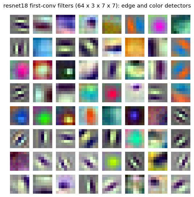
../../_images/9cfe14bc149a30121b38d2c2cf033c87387904c33dd3fd81bb5bb42c158d0eaf.png

What to notice: many filters look like oriented edge detectors (light-dark stripes at various angles) and others are smooth color blobs (opponent red/green, blue/yellow). These are generic, task-agnostic features. Almost every natural-image task benefits from them, which is exactly why they transfer.

3. The transfer learning idea#

Transfer learning: take knowledge learned on a large source task (ImageNet, ~1.2M images, 1000 classes) and reuse it to help a target task that has little labeled data.

A pretrained CNN splits naturally into two parts:

\[\underbrace{\text{conv layers}}_{\text{feature extractor (backbone)}} \;\to\; \underbrace{\text{fully-connected}}_{\text{classifier head}}\]

Two modes of transfer:

(a) Feature extraction: freeze the backbone and train only a new head. The backbone acts as a fixed function that turns an image into a feature vector. Fast, few parameters, resists overfitting.
(b) Fine-tuning: use the pretrained weights as an initialization and keep training some or all layers, usually with a low learning rate so we do not destroy the learned features.

Which to choose depends on how big the target dataset is and how similar it is to the source. We build a decision guide in Section 6.

4. Freezing layers in PyTorch#

Two mechanics do all the work:

Freeze a parameter: set param.requires_grad = False. Frozen params receive no gradient and never update.
Replace the head: swap net.fc (a Linear(512, 1000) for ImageNet) with a fresh Linear(512, K) for your K classes. A newly created layer has requires_grad=True by default, so only the head trains.

resnet18’s body is organized into stages layer1, layer2, layer3, layer4 (increasingly specialized), followed by fc. Unfreezing more of the late stages moves you along a spectrum from pure feature extraction (only fc trains) to full fine-tuning (everything trains).

from torchvision.models import resnet18, ResNet18_Weights

K = 4  # number of target classes for our demo

def make_transfer_model(num_classes=K):
    m = resnet18(weights=ResNet18_Weights.DEFAULT)
    for p in m.parameters():          # freeze the whole backbone
        p.requires_grad = False
    m.fc = nn.Linear(m.fc.in_features, num_classes)  # fresh trainable head
    return m

model = make_transfer_model(K)
tot = count_params(model)
tr  = count_trainable(model)
print(f"Total parameters:     {tot:,}")
print(f"Trainable parameters: {tr:,}  ({100*tr/tot:.3f}% of total)")
print(f"\nOnly the new fc head ({model.fc.in_features} -> {K}) trains; "
      f"the {tot-tr:,} backbone params are frozen.")

Total parameters:     11,178,564
Trainable parameters: 2,052  (0.018% of total)

Only the new fc head (512 -> 4) trains; the 11,176,512 backbone params are frozen.

Widget: unfreeze the last N stages#

Try this: move from none (pure feature extraction) toward all (full fine-tuning) and watch the trainable parameter count and its share of the total grow.

from torchvision.models import resnet18, ResNet18_Weights

# Build once; the widget just toggles requires_grad flags (instant).
_base = resnet18(weights=ResNet18_Weights.DEFAULT)
_base.fc = nn.Linear(_base.fc.in_features, K)
_TOTAL = count_params(_base)

# Ordered from head outward. Each option unfreezes fc plus the listed stages.
UNFREEZE = {
    'none (fc only)':      ['fc'],
    'layer4':              ['fc', 'layer4'],
    'layer3 + layer4':     ['fc', 'layer4', 'layer3'],
    'all (full finetune)': ['fc', 'layer4', 'layer3', 'layer2', 'layer1', 'conv1', 'bn1'],
}

def _unfreeze_demo(scope='none (fc only)'):
    stages = UNFREEZE[scope]
    for name, p in _base.named_parameters():
        p.requires_grad = any(name.startswith(s) for s in stages)
    tr = count_trainable(_base)
    pct = 100 * tr / _TOTAL

    fig, ax = plt.subplots(figsize=(6, 2.6))
    ax.barh([0], [pct], color='#4C72B0')
    ax.set_xlim(0, 100)
    ax.set_yticks([])
    ax.set_xlabel('% of parameters trainable')
    ax.set_title(f"Unfreeze: {scope}\n{tr:,} / {_TOTAL:,} trainable  ({pct:.2f}%)")
    plt.show()

interact(_unfreeze_demo,
         scope=widgets.Dropdown(options=list(UNFREEZE.keys()),
                                value='none (fc only)', description='unfreeze'));

What to notice: fc alone is a tiny fraction of the parameters. layer4 holds most of resnet18’s weights (the widest, most specialized stage), so unfreezing it jumps the trainable share sharply. This is the feature-extraction to fine-tuning spectrum in one control.

5. Hands-on micro-demo: feature extraction on a tiny CIFAR-10 subset#

Plan:

Use the frozen resnet18 up to its global average pool as a fixed feature extractor (output is a 512-dim vector per image).
Extract features once under torch.no_grad() and cache them. This is the expensive step, and we only pay it a single time.
Train a lightweight linear classifier on top of the cached features for a few epochs. This is tiny and fast.
Compare against a small CNN trained from scratch on the same tiny data.

We use a small subset of CIFAR-10: a few classes, about 120 to 150 train and 40 to 50 test images per class, resized to 96x96 and normalized with ImageNet statistics.

from torchvision import datasets, transforms
from torch.utils.data import DataLoader, Subset

CLASSES = [0, 1, 8, 9]          # airplane, automobile, ship, truck (vehicles: a coherent 4-class task)
CLASS_NAMES = ['airplane', 'automobile', 'ship', 'truck']
N_TRAIN_PER = 150               # images per class for training
N_TEST_PER  = 50                # images per class for testing
IMG = 96

imagenet_norm = transforms.Normalize(mean=[0.485, 0.456, 0.406],
                                      std=[0.229, 0.224, 0.225])
tf = transforms.Compose([
    transforms.Resize(IMG),
    transforms.ToTensor(),
    imagenet_norm,
])

train_full = datasets.CIFAR10(root='./data', train=True,  download=True, transform=tf)
test_full  = datasets.CIFAR10(root='./data', train=False, download=True, transform=tf)

remap = {c: i for i, c in enumerate(CLASSES)}   # original label -> 0..K-1

def subset_indices(ds, per_class):
    targets = np.array(ds.targets)
    idx = []
    for c in CLASSES:
        cand = np.where(targets == c)[0][:per_class]
        idx.extend(cand.tolist())
    return idx

train_idx = subset_indices(train_full, N_TRAIN_PER)
test_idx  = subset_indices(test_full,  N_TEST_PER)
train_sub = Subset(train_full, train_idx)
test_sub  = Subset(test_full,  test_idx)
print(f"Classes: {CLASS_NAMES}")
print(f"Train images: {len(train_sub)}   Test images: {len(test_sub)}   (size {IMG}x{IMG})")

Classes: ['airplane', 'automobile', 'ship', 'truck']
Train images: 600   Test images: 200   (size 96x96)

from torchvision.models import resnet18, ResNet18_Weights

# Feature extractor = pretrained resnet18 with its fc removed (identity), frozen and in eval mode.
backbone = resnet18(weights=ResNet18_Weights.DEFAULT)
backbone.fc = nn.Identity()          # output is the 512-dim pooled feature
backbone = backbone.to(device).eval()
for p in backbone.parameters():
    p.requires_grad = False

@torch.no_grad()
def extract_features(subset):
    loader = DataLoader(subset, batch_size=64, shuffle=False)
    feats, labels = [], []
    for xb, yb in loader:
        f = backbone(xb.to(device)).cpu()
        feats.append(f)
        labels.append(torch.tensor([remap[int(y)] for y in yb]))
    return torch.cat(feats), torch.cat(labels)

t0 = time.time()
Xtr, ytr = extract_features(train_sub)   # cache: computed ONCE
Xte, yte = extract_features(test_sub)
print(f"Extracted features in {time.time()-t0:.1f}s")
print("Train feature matrix:", tuple(Xtr.shape), " Test:", tuple(Xte.shape))

Extracted features in 2.5s
Train feature matrix: (600, 512)  Test: (200, 512)

# Train a single Linear head on the cached 512-dim features. This is fast because
# no convolutions run during training: we already cached the features.
def train_linear_head(Xtr, ytr, Xte, yte, num_classes, epochs=40, lr=0.05, seed=0):
    torch.manual_seed(seed)
    head = nn.Linear(Xtr.shape[1], num_classes)
    opt = torch.optim.SGD(head.parameters(), lr=lr, momentum=0.9, weight_decay=1e-4)
    lossf = nn.CrossEntropyLoss()
    for ep in range(epochs):
        head.train()
        opt.zero_grad()
        loss = lossf(head(Xtr), ytr)
        loss.backward()
        opt.step()
    head.eval()
    with torch.no_grad():
        acc = (head(Xte).argmax(1) == yte).float().mean().item()
    return acc, head

t0 = time.time()
feat_acc, _ = train_linear_head(Xtr, ytr, Xte, yte, len(CLASSES))
print(f"Frozen features + linear head test accuracy: {feat_acc*100:.1f}%  "
      f"(trained in {time.time()-t0:.2f}s)")

Frozen features + linear head test accuracy: 87.0%  (trained in 0.03s)

# Baseline: a tiny CNN trained FROM SCRATCH on the same tiny data, comparable budget.
class TinyCNN(nn.Module):
    def __init__(self, num_classes):
        super().__init__()
        self.features = nn.Sequential(
            nn.Conv2d(3, 16, 3, padding=1), nn.ReLU(), nn.MaxPool2d(2),   # 96 -> 48
            nn.Conv2d(16, 32, 3, padding=1), nn.ReLU(), nn.MaxPool2d(2),  # 48 -> 24
            nn.Conv2d(32, 64, 3, padding=1), nn.ReLU(), nn.AdaptiveAvgPool2d(1),
        )
        self.head = nn.Linear(64, num_classes)
    def forward(self, x):
        z = self.features(x).flatten(1)
        return self.head(z)

def train_from_scratch(train_sub, test_sub, num_classes, epochs=12, lr=0.01, seed=0):
    torch.manual_seed(seed)
    net = TinyCNN(num_classes).to(device)
    opt = torch.optim.SGD(net.parameters(), lr=lr, momentum=0.9, weight_decay=1e-4)
    lossf = nn.CrossEntropyLoss()
    tr_loader = DataLoader(train_sub, batch_size=64, shuffle=True)
    for ep in range(epochs):
        net.train()
        for xb, yb in tr_loader:
            yb = torch.tensor([remap[int(y)] for y in yb]).to(device)
            opt.zero_grad()
            loss = lossf(net(xb.to(device)), yb)
            loss.backward(); opt.step()
    net.eval()
    correct = tot = 0
    te_loader = DataLoader(test_sub, batch_size=64)
    with torch.no_grad():
        for xb, yb in te_loader:
            yb = torch.tensor([remap[int(y)] for y in yb]).to(device)
            pred = net(xb.to(device)).argmax(1)
            correct += (pred == yb).sum().item(); tot += len(yb)
    return correct / tot

t0 = time.time()
scratch_acc = train_from_scratch(train_sub, test_sub, len(CLASSES))
print(f"Tiny CNN from scratch test accuracy: {scratch_acc*100:.1f}%  "
      f"(trained in {time.time()-t0:.1f}s)")

Tiny CNN from scratch test accuracy: 40.0%  (trained in 9.4s)

# Compare: from scratch vs frozen features + linear head.
fig, ax = plt.subplots(figsize=(5, 3.2))
names = ['From scratch\n(tiny CNN)', 'Frozen features\n+ linear head']
vals = [scratch_acc*100, feat_acc*100]
bars = ax.bar(names, vals, color=['#C44E52', '#4C72B0'])
ax.set_ylabel('Test accuracy (%)')
ax.set_ylim(0, 100)
ax.axhline(100/len(CLASSES), ls='--', color='gray', lw=1)
ax.text(1.4, 100/len(CLASSES)+2, 'chance', color='gray', ha='right', fontsize=8)
for b, v in zip(bars, vals):
    ax.text(b.get_x()+b.get_width()/2, v+1.5, f'{v:.0f}%', ha='center')
ax.set_title('Transfer learning wins on tiny data')
plt.show()

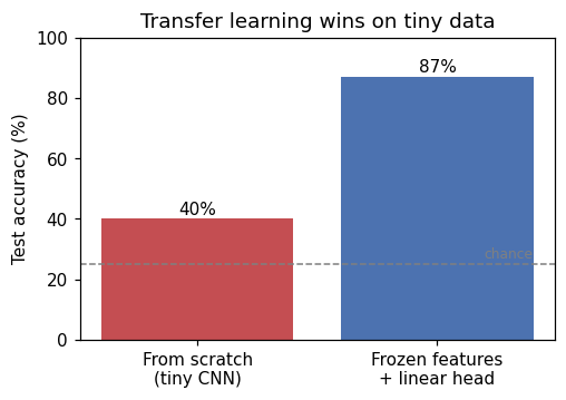
../../_images/11e6b86f7db727d1eef5378603475fb463a71fba84b1b223d98f119752549fb6.png

What to notice: with only a few hundred images, the from-scratch CNN struggles (little data, random init), while frozen pretrained features + a linear head reaches much higher accuracy in a fraction of the time. The pretrained backbone already knows how to see; we only teach it a new decision rule.

Widget: data-efficiency curve#

We already cached the full feature matrix, so this widget just subsamples the cached features and retrains the fast linear head. No convolutions rerun, so it is instant.

Try this: drop to just a handful of images per class and see that transfer still works far above chance. This is the practical payoff: transfer learning is data-efficient.

# Precompute a per-class index list into the cached training features for fast subsampling.
_by_class = {c: (ytr == c).nonzero(as_tuple=True)[0] for c in range(len(CLASSES))}

def _data_efficiency(n_per_class=150):
    g = torch.Generator().manual_seed(0)
    sel = []
    for c in range(len(CLASSES)):
        pool = _by_class[c]
        k = min(n_per_class, len(pool))
        perm = torch.randperm(len(pool), generator=g)[:k]
        sel.append(pool[perm])
    sel = torch.cat(sel)
    acc, _ = train_linear_head(Xtr[sel], ytr[sel], Xte, yte, len(CLASSES))

    fig, ax = plt.subplots(figsize=(5, 3))
    ax.bar([0], [acc*100], color='#4C72B0', width=0.5)
    ax.set_xlim(-1, 1); ax.set_ylim(0, 100); ax.set_xticks([])
    ax.axhline(100/len(CLASSES), ls='--', color='gray', lw=1)
    ax.set_ylabel('Test accuracy (%)')
    ax.set_title(f'{n_per_class} imgs/class  ->  {acc*100:.1f}% test acc')
    plt.show()

interact(_data_efficiency,
         n_per_class=widgets.IntSlider(min=5, max=N_TRAIN_PER, step=5,
                                       value=N_TRAIN_PER, description='imgs/class'));

6. Decision guide: which strategy to use#

The practical heart of the lecture is a 2x2 matrix over dataset size (small vs large) and domain similarity to ImageNet (similar vs dissimilar):

	Similar domain	Dissimilar domain
Small data	Freeze the backbone, train only a linear classifier (prevents overfitting).	Take features from an earlier layer (more generic) and train a simple classifier (linear or SVM).
Large data	Fine-tune the whole network, using pretrained weights as a strong initialization.	Fine-tune the whole network; if very different, consider training from scratch.

Intuition:

Little data means few trainable parameters, so favor freezing to avoid overfitting.
Dissimilar domain means the specialized late features do not transfer, so rely on the generic early features.
Lots of data means you can afford to update many parameters, so fine-tune broadly.

Widget: pick your situation, get a recommendation#

Try this: set the two dropdowns to your real-world scenario and read off the recommended strategy.

RECS = {
    ('small', 'similar'): (
        "Freeze the backbone; train ONLY a linear classifier head.",
        "Few labels + similar features: freezing avoids overfitting and reuses the pretrained features directly."),
    ('small', 'dissimilar'): (
        "Use features from an EARLIER layer; train a simple classifier (linear or SVM).",
        "Late features are ImageNet-specific and will not transfer; early features are generic and still useful."),
    ('large', 'similar'): (
        "Fine-tune the WHOLE network with a low learning rate.",
        "Enough data to update all layers safely; pretrained weights give a strong initialization."),
    ('large', 'dissimilar'): (
        "Fine-tune the whole network; if the domain is very different, consider training from scratch.",
        "Plenty of data can adapt even specialized layers; a very different domain may need fresh features."),
}

def _decide(dataset_size='small', similarity='similar'):
    strategy, reason = RECS[(dataset_size, similarity)]
    print(f"Situation : {dataset_size} data, {similarity} domain")
    print("-" * 60)
    print("Strategy  :", strategy)
    print("Why       :", reason)

interact(_decide,
         dataset_size=widgets.Dropdown(options=['small', 'large'], value='small',
                                       description='data size'),
         similarity=widgets.Dropdown(options=['similar', 'dissimilar'], value='similar',
                                     description='similarity'));

7. Fine-tuning tips#

When you do choose to fine-tune (not just feature-extract):

Use a low learning rate. A large step would wash out the carefully learned pretrained features before they can help.
Discriminative learning rates. Give early layers a smaller LR (they are generic, change them little) and the head a larger LR (it is new and must learn fast). Implement this with parameter groups.
Data augmentation. Random crops, flips, and color jitter enlarge a small dataset and reduce overfitting during fine-tuning.

Below is the standard pattern: build one optimizer with two param groups, a small LR for the backbone and a larger LR for the head.

from torchvision.models import resnet18, ResNet18_Weights

ft = resnet18(weights=ResNet18_Weights.DEFAULT)
ft.fc = nn.Linear(ft.fc.in_features, K)   # fresh head for K classes

backbone_params = [p for n, p in ft.named_parameters() if not n.startswith('fc')]
head_params     = [p for n, p in ft.named_parameters() if n.startswith('fc')]

optimizer = torch.optim.SGD([
    {'params': backbone_params, 'lr': 1e-4},   # small LR: preserve pretrained features
    {'params': head_params,     'lr': 1e-2},   # larger LR: learn the new head fast
], momentum=0.9, weight_decay=1e-4)

# Example augmentation pipeline you would use for the training data.
aug = transforms.Compose([
    transforms.RandomResizedCrop(IMG, scale=(0.7, 1.0)),
    transforms.RandomHorizontalFlip(),
    transforms.ColorJitter(0.2, 0.2, 0.2),
    transforms.ToTensor(),
    imagenet_norm,
])

for i, grp in enumerate(optimizer.param_groups):
    n = sum(p.numel() for p in grp['params'])
    print(f"param group {i}: lr={grp['lr']:<7} params={n:,}")
print("\nBackbone updates slowly, head updates quickly: discriminative learning rates.")

param group 0: lr=0.0001  params=11,176,512
param group 1: lr=0.01    params=2,052

Backbone updates slowly, head updates quickly: discriminative learning rates.

Key takeaways#

Training deep CNNs from scratch is hard: fragile optimization, easy overfitting on small data, and large compute cost.
CNN features are hierarchical: early layers are generic (edges, colors) and transfer widely; late layers are specialized to the source task.
Transfer learning reuses a network pretrained on a large source (ImageNet) for a small target task.
Two modes: feature extraction (freeze backbone, train a new head) and fine-tuning (keep training with a low LR). In PyTorch, control this with requires_grad and by replacing fc.
On tiny data, frozen features + a linear head beat a from-scratch CNN, and stay strong even with very few labels.
Pick your strategy from the size x similarity matrix: small data favors freezing; dissimilar domains favor earlier (more generic) features; large data allows full fine-tuning.

Exercises#

Freeze depth versus accuracy. Freeze everything, then progressively unfreeze layer4, layer3, layer2. Plot trainable parameter count against accuracy on a small target set and find where the returns stop.
Learning rate matters more when fine-tuning. Sweep the learning rate for feature extraction and for full fine-tuning. Explain why the best value is much smaller in the second case.
Swap the head correctly. Replace fc with a fresh Linear(512, K) and verify by inspecting requires_grad that only the head receives gradients.
Pick the strategy from the data. Construct a very small target set and a larger one, and show which of feature extraction or fine-tuning wins in each case.