Week 3, Lecture 8: Early Stopping, Data Augmentation, Noise, Ensembles, and Dropout

Week 3, Lecture 8: Early Stopping, Data Augmentation, Noise, Ensembles, and Dropout#

NPTEL Deep Learning for Computer Vision | Prof. Vineeth N Balasubramanian, IIT Hyderabad

Companion notebook for §3.4 Regularization in Neural Networks.

We build each regularizer bottom-up in PyTorch on tiny, bundled datasets, and use interactive sliders so you can feel how each knob behaves.

What you will learn

Early stopping: watch validation error and stop before it overfits, using a patience rule.
Data augmentation: label-preserving image transforms (rotation, flip, additive noise, CutOut, Mixup).
Noise injection: zero-mean Gaussian input noise as a regularizer (equivalent to L2 weight decay under MSE).
Ensembles / bagging: average $k$ bootstrap models and match the theory $\frac{1}{k}V + \frac{k-1}{k}C$.
Dropout from scratch: inverted dropout, verified against nn.Dropout, narrowing the train/validation gap.

How to run Works on Colab (CPU or GPU) or a local Jupyter install. Every dataset here is tiny and bundled with scikit-learn (load_digits), so there are no downloads and the whole notebook runs in well under a minute on CPU. Run the setup cell below first, then go top to bottom.

Contents

Early stopping
Data augmentation on images
Noise injection as regularization
Ensembles and bagging
Dropout, from scratch

Review#

The previous lecture made overfitting visible with polynomial regression, compared Lp norm geometry, and derived L2 weight decay along with its eigen-analysis. L2 is one regularizer among many. This lecture builds the rest.

Setup#

# Run this cell first. Works on Colab (CPU or GPU) and local Jupyter.
import sys, subprocess
# ipywidgets ships with Colab; install only if it is missing.
try:
    import ipywidgets  # noqa: F401
except ImportError:
    subprocess.run([sys.executable, "-m", "pip", "install", "-q", "ipywidgets"])

import numpy as np
import torch
import torch.nn as nn
import torch.nn.functional as F
import matplotlib.pyplot as plt
from ipywidgets import interact, interactive, FloatSlider, IntSlider, Dropdown, Checkbox, fixed
%matplotlib inline

# Reproducibility
torch.manual_seed(0)
np.random.seed(0)

# Use a GPU if one is available, otherwise CPU. Every demo here is tiny and
# runs in seconds on CPU, so no GPU is required.
device = torch.device("cuda" if torch.cuda.is_available() else "cpu")

plt.rcParams["figure.figsize"] = (7, 4.5)
plt.rcParams["axes.grid"] = True
plt.rcParams["axes.axisbelow"] = True

print("PyTorch", torch.__version__, "| device:", device)

PyTorch 2.8.0 | device: cpu

1. Early stopping#

The simplest regularizer: keep monitoring the validation error and stop before the model starts overfitting the training set. As training proceeds, training loss keeps dropping, but validation loss decreases, bottoms out, then turns back up. The bottom of that U is where we want to stop.

When to stop? A fixed “train $n$ epochs, drop the learning rate, train $m$ more” schedule is a bad idea: one size does not fit all. The slides give two data-driven criteria:

Error-change criterion: stop when the validation error has not dropped over a window of, say, $10$ epochs. This is exactly the “patience” idea below. After the criterion triggers, one often trains a few more epochs at a lower learning rate.
Weight-change criterion: compare the weights at epochs $t-10$ and $t$ and stop when $\max_i \| w_i^{t} - w_i^{t-10} \| < \rho$ (per-weight, not the length of the whole change vector, possibly as a percentage of the weight).

We first train a wide MLP on a deliberately tiny slice of the 8x8 digits so it overfits, recording train and validation loss every epoch. We train once, then replay the recorded curve to apply the stopping rule (this keeps the widget fast).

from sklearn.datasets import load_digits
from sklearn.model_selection import train_test_split

# 8x8 handwritten digits: 1797 images, 10 classes. Bundled with sklearn, no download.
digits = load_digits()
X_all = digits.data.astype(np.float32) / 16.0   # pixel range scaled to 0 to 1
y_all = digits.target.astype(np.int64)

# TINY training set so a wide MLP can memorize it, plus a larger validation set
# so we can watch validation loss turn back up (overfitting).
Xtr, Xval, ytr, yval = train_test_split(
    X_all, y_all, train_size=120, test_size=500, random_state=0, stratify=y_all)

Xtr_t = torch.tensor(Xtr, device=device)
ytr_t = torch.tensor(ytr, device=device)
Xval_t = torch.tensor(Xval, device=device)
yval_t = torch.tensor(yval, device=device)

def make_mlp(in_dim=64, hidden=64, out_dim=10):
    return nn.Sequential(
        nn.Linear(in_dim, hidden), nn.ReLU(),
        nn.Linear(hidden, hidden), nn.ReLU(),
        nn.Linear(hidden, out_dim),
    )

torch.manual_seed(0)
es_model = make_mlp().to(device)
opt = torch.optim.Adam(es_model.parameters(), lr=5e-3)
lossf = nn.CrossEntropyLoss()

n_epochs = 250
es_train_loss, es_val_loss = [], []
for ep in range(n_epochs):
    es_model.train()
    opt.zero_grad()
    loss = lossf(es_model(Xtr_t), ytr_t)
    loss.backward()
    opt.step()
    es_model.eval()
    with torch.no_grad():
        vloss = lossf(es_model(Xval_t), yval_t)
    es_train_loss.append(loss.item())
    es_val_loss.append(vloss.item())

es_train_loss = np.array(es_train_loss)
es_val_loss = np.array(es_val_loss)
best_epoch = int(np.argmin(es_val_loss))
print("Trained %d epochs on %d samples." % (n_epochs, len(ytr)))
print("Best (lowest-validation) epoch: %d | validation loss there: %.4f" %
      (best_epoch, es_val_loss[best_epoch]))

Trained 250 epochs on 120 samples.
Best (lowest-validation) epoch: 26 | validation loss there: 0.4333

The patience rule (error-change criterion)#

We keep the best validation loss seen so far. Each epoch that fails to improve on it increments a wait counter; once wait reaches patience, we stop and restore the weights from the best epoch. A small patience stops early (risking stopping on a noisy bump); a large patience lets training run longer (risking overfitting). Move the slider to see the trade-off on the recorded curve.

def early_stop_point(val_losses, patience):
    """Replay a recorded validation curve with the error-change rule: stop once
    validation loss has not improved for `patience` epochs. Returns the epoch we
    stop at and the best (lowest-validation) epoch seen up to that point."""
    best, best_ep, wait = np.inf, 0, 0
    for ep, v in enumerate(val_losses):
        if v < best:
            best, best_ep, wait = v, ep, 0
        else:
            wait += 1
            if wait >= patience:
                return ep, best_ep
    return len(val_losses) - 1, best_ep

def show_early_stopping(patience=10):
    stop_ep, best_ep = early_stop_point(es_val_loss, patience)
    plt.figure()
    plt.plot(es_train_loss, label="train loss")
    plt.plot(es_val_loss, label="validation loss")
    plt.axvline(stop_ep, color="red", ls="--", label="stop at epoch %d" % stop_ep)
    plt.scatter([best_ep], [es_val_loss[best_ep]], color="black", zorder=5,
                label="best epoch %d" % best_ep)
    plt.xlabel("epoch")
    plt.ylabel("cross-entropy loss")
    plt.title("Early stopping with patience = %d epochs" % patience)
    plt.legend()
    plt.show()
    print("Stop at epoch %d, restore weights from epoch %d (validation loss %.4f)." %
          (stop_ep, best_ep, es_val_loss[best_ep]))

# WIDGET: patience -> where training stops and the resulting validation error.
interact(show_early_stopping,
         patience=IntSlider(min=1, max=50, step=1, value=10));

2. Data augmentation on images#

Idea: create more training data by applying transformations that do not change the label. This both grows a small dataset and acts as a regularizer by discouraging the network from overfitting the exact pixels it was given.

Classic transforms (from the slide): data jittering (distortion / blur), rotations, color changes, additive noise, and mirroring (horizontal flip).

Newer methods:

Mixup: build virtual examples by blending two samples with $\lambda \in [0,1]$: $$\tilde{x} = \lambda x_i + (1-\lambda) x_j, \qquad \tilde{y} = \lambda y_i + (1-\lambda) y_j$$ where $y_i, y_j$ are one-hot labels. Variants: Manifold Mixup, AugMix.
CutOut: randomly mask out (zero) a square region of the input during training. Variant: CutMix.

We implement each transform from scratch on numpy arrays using one 8x8 digit (an image of a “0”), plus a second digit (a “7”) for Mixup.

from scipy.ndimage import rotate as nd_rotate

# One 8x8 sample image, plus a second (different class) for Mixup.
# digits.images is 1797 x 8 x 8.
img_a = digits.images[0].astype(np.float32) / 16.0                 # a "0"
idx_b = int(np.where(digits.target == 7)[0][0])
img_b = digits.images[idx_b].astype(np.float32) / 16.0            # a "7"

def aug_rotate(img, angle):
    r = nd_rotate(img, angle, reshape=False, order=1, mode="constant", cval=0.0)
    return np.clip(r, 0.0, 1.0)

def aug_flip(img):
    return np.fliplr(img).copy()                                  # mirroring

def aug_noise(img, sigma, seed=0):
    rng = np.random.RandomState(seed)
    return np.clip(img + sigma * rng.randn(*img.shape), 0.0, 1.0)  # additive jitter

def aug_cutout(img, size, seed=0):
    rng = np.random.RandomState(seed)
    out = img.copy()
    h, w = img.shape
    if size > 0:
        cy, cx = rng.randint(0, h), rng.randint(0, w)
        y0, y1 = max(0, cy - size // 2), min(h, cy + (size + 1) // 2)
        x0, x1 = max(0, cx - size // 2), min(w, cx + (size + 1) // 2)
        out[y0:y1, x0:x1] = 0.0                                   # mask a square
    return out

def aug_mixup(img1, img2, lam):
    return lam * img1 + (1.0 - lam) * img2                        # blend two digits

# Static grid: original plus one example of each augmentation.
panels = [
    ("original", img_a),
    ("rotate 30 deg", aug_rotate(img_a, 30)),
    ("horizontal flip", aug_flip(img_a)),
    ("additive noise", aug_noise(img_a, 0.3)),
    ("cutout", aug_cutout(img_a, 3)),
    ("mixup lam=0.5", aug_mixup(img_a, img_b, 0.5)),
]
fig, axes = plt.subplots(2, 3, figsize=(8, 5.5))
for ax, (title, im) in zip(axes.ravel(), panels):
    ax.imshow(im, cmap="gray_r", vmin=0, vmax=1)
    ax.set_title(title)
    ax.set_xticks([]); ax.set_yticks([]); ax.grid(False)
fig.suptitle("Label-preserving augmentations of one 8x8 digit")
plt.show()

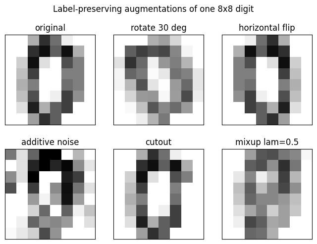
../../_images/2de71f5e5d135c0726d071b19b0f0bfcdb714fc986b5ad8bee67110e96936d96.png

Now make it live. The sliders redraw the augmented digit as you change the rotation angle, the CutOut square size, and the Mixup weight $\lambda$ (which blends the “0” toward the “7”).

def show_augment(angle=30, cutout_size=3, mixup_lam=0.5):
    views = [
        ("original", img_a),
        ("rotate %d deg" % angle, aug_rotate(img_a, angle)),
        ("cutout size %d" % cutout_size, aug_cutout(img_a, cutout_size)),
        ("mixup lam=%.2f" % mixup_lam, aug_mixup(img_a, img_b, mixup_lam)),
    ]
    fig, axes = plt.subplots(1, 4, figsize=(10, 3))
    for ax, (title, im) in zip(axes, views):
        ax.imshow(im, cmap="gray_r", vmin=0, vmax=1)
        ax.set_title(title)
        ax.set_xticks([]); ax.set_yticks([]); ax.grid(False)
    fig.suptitle("Augmentation controls")
    plt.show()

# WIDGET: rotation angle, cutout size, and mixup lambda redraw the image live.
interact(show_augment,
         angle=IntSlider(min=-90, max=90, step=15, value=30),
         cutout_size=IntSlider(min=0, max=6, step=1, value=3),
         mixup_lam=FloatSlider(min=0.0, max=1.0, step=0.05, value=0.5));

3. Noise injection as regularization#

Injecting noise during training is another form of regularization. The slide lists three flavors:

Data noise: add noise to the inputs while training. A classic result (Bishop, 1995) is that adding zero-mean Gaussian noise to the input is equivalent to L2 weight decay (Tikhonov regularization) when the loss is sum-of-squared error (MSE). It can also be seen as a form of data augmentation.
Label noise (DisturbLabel): with probability $\alpha$, replace a sample’s label with one drawn uniformly from $\{1, \dots, C\}$, ignoring the true label.
Gradient noise: perturb the gradient, $g_t \leftarrow g_t + \mathcal{N}(0, \sigma_t^2)$, with an annealed variance $\sigma_t^2 = \frac{\eta}{(1+t)^\gamma}$.

We demonstrate data noise: fit a small MLP to a few noisy 1D points, adding fresh Gaussian input noise each step. With no noise the fit is wiggly (it chases each point); as the noise level $\sigma$ grows, the fit smooths out, which is exactly the L2-style regularization effect.

def true_fn(x):
    return np.sin(2.5 * x) + 0.4 * x

rng = np.random.RandomState(1)
x_train = np.linspace(-2.5, 2.5, 18).astype(np.float32)
y_train = (true_fn(x_train) + 0.15 * rng.randn(len(x_train))).astype(np.float32)
x_grid = np.linspace(-3.0, 3.0, 200).astype(np.float32)

xt = torch.tensor(x_train, device=device).view(-1, 1)
yt = torch.tensor(y_train, device=device).view(-1, 1)
xg = torch.tensor(x_grid, device=device).view(-1, 1)

def fit_with_input_noise(sigma=0.0, epochs=400, seed=0):
    torch.manual_seed(seed)
    net = nn.Sequential(nn.Linear(1, 64), nn.Tanh(),
                        nn.Linear(64, 64), nn.Tanh(),
                        nn.Linear(64, 1)).to(device)
    opt = torch.optim.Adam(net.parameters(), lr=1e-2)
    lossf = nn.MSELoss()
    for _ in range(epochs):
        opt.zero_grad()
        xin = xt + sigma * torch.randn_like(xt)   # zero-mean Gaussian input noise
        loss = lossf(net(xin), yt)
        loss.backward()
        opt.step()
    net.eval()
    with torch.no_grad():
        return net(xg).cpu().numpy().ravel()

def show_noise_reg(sigma=0.0):
    yg = fit_with_input_noise(sigma=sigma)
    plt.figure()
    plt.plot(x_grid, true_fn(x_grid), "k--", label="true function")
    plt.scatter(x_train, y_train, color="tab:blue", label="training points")
    plt.plot(x_grid, yg, color="tab:red", label="MLP fit")
    plt.xlabel("x"); plt.ylabel("y")
    plt.title("Input-noise regularization: sigma = %.2f" % sigma)
    plt.legend(); plt.ylim(-3, 3)
    plt.show()

# WIDGET: input-noise sigma -> smoothness of the fitted curve.
interact(show_noise_reg,
         sigma=FloatSlider(min=0.0, max=1.0, step=0.05, value=0.0));

4. Ensembles and bagging#

Bagging (bootstrap aggregating): build $k$ training sets by sampling the data with replacement, train one model on each, and average their predictions.

Why it helps (the slide’s derivation). Suppose model $i$ makes error $\varepsilon_i$ on a test example, drawn zero-mean with variance $V = \mathbb{E}[\varepsilon_i^2]$ and covariance $C = \mathbb{E}[\varepsilon_i \varepsilon_j]$. The average prediction has error $\frac{1}{k}\sum_i \varepsilon_i$, whose expected squared error is $$\mathrm{MSE} = \mathbb{E}\Big[\Big(\tfrac{1}{k}\textstyle\sum_i \varepsilon_i\Big)^2\Big] = \frac{1}{k}V + \frac{k-1}{k}C .$$

If errors are perfectly correlated ($C = V$), then $\mathrm{MSE} = V$: bagging does not help.
If errors are independent ($C = 0$), then $\mathrm{MSE} = \frac{1}{k}V$: error falls off as $1/k$.
In general the error floor is $C$, the shared (correlated) part of the error.

We train $k$ small MLPs, each on its own bootstrap resample of a noisy 1D dataset, measure $V$ and $C$ empirically from the per-model errors, and check that the measured ensemble error follows the theory curve.

rng = np.random.RandomState(2)
N = 40
xb = np.linspace(-3.0, 3.0, N).astype(np.float32)
yb = (np.sin(1.5 * xb) + 0.3 * rng.randn(N)).astype(np.float32)
xtest = np.linspace(-3.0, 3.0, 100).astype(np.float32)
ytest = np.sin(1.5 * xtest).astype(np.float32)          # clean test targets
xtest_t = torch.tensor(xtest, device=device).view(-1, 1)

K_MAX = 20
def train_member(seed):
    g = np.random.RandomState(seed)
    idx = g.randint(0, N, size=N)                       # bootstrap: sample with replacement
    xi = torch.tensor(xb[idx], device=device).view(-1, 1)
    yi = torch.tensor(yb[idx], device=device).view(-1, 1)
    torch.manual_seed(seed)
    net = nn.Sequential(nn.Linear(1, 16), nn.Tanh(),
                        nn.Linear(16, 16), nn.Tanh(),
                        nn.Linear(16, 1)).to(device)
    opt = torch.optim.Adam(net.parameters(), lr=1e-2)
    lossf = nn.MSELoss()
    for _ in range(300):
        opt.zero_grad()
        loss = lossf(net(xi), yi)
        loss.backward()
        opt.step()
    net.eval()
    with torch.no_grad():
        return net(xtest_t).cpu().numpy().ravel()

preds = np.stack([train_member(s) for s in range(K_MAX)])   # K_MAX x 100
errs = preds - ytest[None, :]                               # per-model test errors

# Empirical variance V and covariance C of the errors (slide's definitions).
V_hat = float(np.mean(errs ** 2))
G = errs @ errs.T                                           # G[i,j] = sum_t eps_i eps_j
offdiag_sum = G.sum() - np.trace(G)                         # sum over i != j
C_hat = float(offdiag_sum / (K_MAX * (K_MAX - 1)) / len(xtest))

ks = np.arange(1, K_MAX + 1)
# Measured ensemble MSE at each k, averaged over random member subsets to smooth it.
sub_rng = np.random.RandomState(3)
emp_mse = []
for k in ks:
    vals = [np.mean((preds[sub_rng.choice(K_MAX, size=k, replace=False)].mean(0) - ytest) ** 2)
            for _ in range(30)]
    emp_mse.append(np.mean(vals))
emp_mse = np.array(emp_mse)
theory_mse = V_hat / ks + (ks - 1) / ks * C_hat

print("Empirical error variance V = %.4f | covariance C = %.4f" % (V_hat, C_hat))
print("As k grows, ensemble error falls toward the covariance floor C.")

Empirical error variance V = 0.0403 | covariance C = 0.0146
As k grows, ensemble error falls toward the covariance floor C.

def show_bagging(k=1):
    plt.figure()
    plt.plot(ks, theory_mse, "k--", label="theory: V/k + (k-1)/k * C")
    plt.plot(ks, emp_mse, "o-", color="tab:blue", label="measured ensemble MSE")
    plt.scatter([k], [emp_mse[k - 1]], color="tab:red", zorder=5,
                label="k = %d, MSE = %.4f" % (k, emp_mse[k - 1]))
    plt.axhline(V_hat, color="tab:green", ls=":", label="single-model level V")
    plt.axhline(C_hat, color="tab:purple", ls=":", label="covariance floor C")
    plt.xlabel("number of ensemble members k")
    plt.ylabel("test MSE")
    plt.title("Bagging: ensemble error vs number of models")
    plt.legend()
    plt.show()

# WIDGET: number of ensemble members k -> error reduction.
interact(show_bagging, k=IntSlider(min=1, max=K_MAX, step=1, value=1));

5. Dropout, from scratch#

Co-adaptation problem: as a large network trains, a few strong connections dominate and weaker units are ignored, so many units end up doing little. Dropout fixes this by forcing units to work without relying on any specific neighbor.

Training phase: for each layer, each sample, each step, randomly zero out a fraction $p$ of the units (and their activations).
Test phase: use all units, but scale activations to compensate for the units that were dropped during training.

Dropout approximates an ensemble of $2^H$ subnetworks ($H$ droppable units) that all share weights, which is what makes it a cheap ensemble and a regularizer.

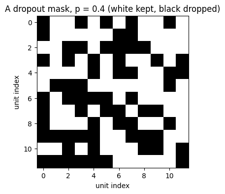
We (1) implement dropout from scratch with a Bernoulli mask and inverted scaling, (2) show it matches PyTorch nn.Dropout in expectation, then (3) drop it into a small MLP and watch it narrow the train/validation gap.

We use inverted dropout (what PyTorch does): keep each unit with probability $1-p$ and divide the survivors by $1-p$ during training, so the expected activation is unchanged and test time is a plain forward pass (identity).

def my_dropout(x, p, training=True):
    """Inverted dropout from scratch.
    TRAIN: keep each unit with prob (1-p), zero the rest, and scale survivors by
    1/(1-p) so the expected activation is unchanged. TEST: identity pass."""
    if not training or p == 0.0:
        return x
    keep = 1.0 - p
    mask = (torch.rand_like(x) < keep).float()
    return x * mask / keep

# Verify our dropout matches nn.Dropout: (1) it preserves the expectation (both
# average back to the original ~1.0 over many draws), and (2) a single draw zeros
# a fraction ~ p of the units, just like nn.Dropout.
torch.manual_seed(0)
x = torch.ones(1000, 64)
p = 0.4
ref_layer = nn.Dropout(p); ref_layer.train()
ours_mean = torch.stack([my_dropout(x, p, training=True) for _ in range(200)]).mean(0).mean().item()
ref_mean = torch.stack([ref_layer(x) for _ in range(200)]).mean(0).mean().item()
drop_ours = (my_dropout(x, p, training=True) == 0).float().mean().item()
drop_ref = (ref_layer(x) == 0).float().mean().item()
print("expectation preserved: mean(ours) = %.3f, mean(nn.Dropout) = %.3f (target 1.0)" %
      (ours_mean, ref_mean))
print("drop fraction in one draw: ours = %.3f, nn.Dropout = %.3f (target p = %.2f)" %
      (drop_ours, drop_ref, p))

# Visualize one dropout mask (white = kept, black = dropped).
torch.manual_seed(1)
mask_vis = (torch.rand(12, 12) < (1 - 0.4)).float().numpy()
plt.figure(figsize=(4, 4))
plt.imshow(mask_vis, cmap="gray", vmin=0, vmax=1)
plt.title("A dropout mask, p = 0.4 (white kept, black dropped)")
plt.xlabel("unit index"); plt.ylabel("unit index"); plt.grid(False)
plt.show()

expectation preserved: mean(ours) = 1.000, mean(nn.Dropout) = 1.000 (target 1.0)
drop fraction in one draw: ours = 0.401, nn.Dropout = 0.400 (target p = 0.40)

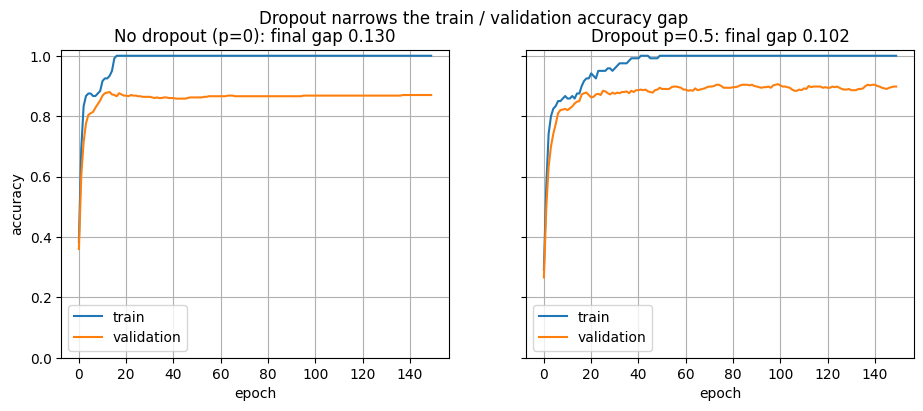
../../_images/fc4f138cfd67612eecae48356cda6943c887aa5ee81a056f718eb869f06ec3ce.png

Now put my_dropout inside an MLP (dropout active only when self.training is True) and train it on the same tiny digits split from section 1, which overfits badly without regularization. We compare no dropout ($p=0$) against dropout ($p=0.5$): dropout lowers the training accuracy a bit but keeps validation accuracy up, shrinking the gap between them.

class DropoutMLP(nn.Module):
    def __init__(self, p=0.5, in_dim=64, hidden=128, out_dim=10):
        super().__init__()
        self.fc1 = nn.Linear(in_dim, hidden)
        self.fc2 = nn.Linear(hidden, hidden)
        self.fc3 = nn.Linear(hidden, out_dim)
        self.p = p

    def forward(self, x):
        x = F.relu(self.fc1(x))
        x = my_dropout(x, self.p, training=self.training)   # from-scratch dropout
        x = F.relu(self.fc2(x))
        x = my_dropout(x, self.p, training=self.training)
        return self.fc3(x)

def train_dropout_mlp(p, epochs=150, seed=0):
    torch.manual_seed(seed)
    model = DropoutMLP(p=p).to(device)
    opt = torch.optim.Adam(model.parameters(), lr=5e-3)
    lossf = nn.CrossEntropyLoss()
    tr_acc, te_acc = [], []
    for ep in range(epochs):
        model.train()
        opt.zero_grad()
        loss = lossf(model(Xtr_t), ytr_t)
        loss.backward()
        opt.step()
        model.eval()
        with torch.no_grad():
            tr = (model(Xtr_t).argmax(1) == ytr_t).float().mean().item()
            te = (model(Xval_t).argmax(1) == yval_t).float().mean().item()
        tr_acc.append(tr); te_acc.append(te)
    return np.array(tr_acc), np.array(te_acc)

tr0, te0 = train_dropout_mlp(0.0)
trd, ted = train_dropout_mlp(0.5)
fig, ax = plt.subplots(1, 2, figsize=(11, 4), sharey=True)
ax[0].plot(tr0, label="train"); ax[0].plot(te0, label="validation")
ax[0].set_title("No dropout (p=0): final gap %.3f" % (tr0[-1] - te0[-1]))
ax[1].plot(trd, label="train"); ax[1].plot(ted, label="validation")
ax[1].set_title("Dropout p=0.5: final gap %.3f" % (trd[-1] - ted[-1]))
for a in ax:
    a.set_xlabel("epoch"); a.set_ylim(0, 1.02); a.legend()
ax[0].set_ylabel("accuracy")
fig.suptitle("Dropout narrows the train / validation accuracy gap")
plt.show()

../../_images/15905249e852ae5ca5654c26cd0830d53cb6169a77b20041f24dcbf0d328dec4.png

def show_dropout(p=0.0):
    tr_acc, te_acc = train_dropout_mlp(p)
    gap = tr_acc[-1] - te_acc[-1]
    plt.figure()
    plt.plot(tr_acc, label="train accuracy")
    plt.plot(te_acc, label="validation accuracy")
    plt.xlabel("epoch"); plt.ylabel("accuracy")
    plt.title("Dropout p = %.2f | final train/validation gap = %.3f" % (p, gap))
    plt.legend(); plt.ylim(0, 1.02)
    plt.show()

# WIDGET: dropout probability p -> train/validation curves and the final gap.
interact(show_dropout,
         p=FloatSlider(min=0.0, max=0.8, step=0.1, value=0.0));

Key takeaways#

Early stopping treats “when to stop” as a hyperparameter chosen by watching validation error. The error-change (patience) and weight-change criteria both aim for the bottom of the validation U; a few extra epochs at a lower learning rate can help afterward.
Data augmentation manufactures label-preserving variants (rotation, flip, jitter, CutOut, Mixup). It enlarges small datasets and regularizes at the same time.
Noise injection regularizes through data noise, label noise (DisturbLabel), or gradient noise. Zero-mean Gaussian input noise smooths the fit and is equivalent to L2 weight decay under MSE.
Bagging averages $k$ bootstrap models; expected error is $\frac{1}{k}V + \frac{k-1}{k}C$. Independent errors give a $1/k$ speedup; correlated errors ($C \to V$) give no gain, and $C$ is the error floor.
Dropout breaks co-adaptation by randomly zeroing units in training and scaling at test time. It behaves like a weight-sharing ensemble of $2^H$ subnetworks and narrows the train/validation gap.

Exercises#

prove the slide’s claim, that adding zero-mean Gaussian noise to the input is equivalent to L2 weight decay when the loss is MSE. Sketch: expand the squared error around the noiseless input, take the expectation over the noise, and identify the extra term as a penalty proportional to the squared weights. Then re-run section 3 and check that raising $\sigma$ behaves like raising a weight-decay coefficient.