
📺 Lecture video | 📄 Slides
Week 3, Lecture 4: Backpropagation, Built by Hand and Verified#
NPTEL Deep Learning for Computer Vision | Prof. Vineeth N Balasubramanian, IIT Hyderabad
Companion notebook for §3.2 Feedforward Networks and Backpropagation.
We build the backpropagation algorithm from the ground up and check it against autograd.
What you will learn
The chain rule on a tiny scalar computation graph, node by node.
A from-scratch forward and backward pass for a 2-layer MLP using only torch tensor math (no autograd).
A proof that our hand-derived gradients match PyTorch autograd to about \(10^{-15}\): backprop is exactly what autograd computes.
Manual gradient descent training on a 2D toy dataset (make_moons), with a live decision boundary.
The same task in idiomatic PyTorch (nn.Module plus an optimizer) to confirm the two agree.
How we build it Primitive pieces first (the scalar chain rule), then the full network from scratch with plain tensors, then the idiomatic PyTorch version, checking agreement at every step.
How to run Colab CPU or GPU, or a local Jupyter. Everything is tiny and finishes in a few seconds on CPU. Run the setup cell first.
Contents
The chain rule on a scalar computation graph
A 2-layer MLP, forward and backward from scratch
The payoff, verify against autograd
Train the from-scratch network with manual gradient descent
The same task, idiomatic PyTorch
Review#
The previous lecture built a feedforward network as a composition of functions and trained it by gradient descent. It relied on gradients we did not derive. This lecture derives them properly with the chain rule, and checks the result against autograd.
Setup#
# Run this cell first. Works on Colab (CPU or GPU) and local Jupyter.
import sys, subprocess
# ipywidgets ships with Colab; install only if it is missing.
try:
    import ipywidgets  # noqa: F401
except ImportError:
    subprocess.run([sys.executable, "-m", "pip", "install", "-q", "ipywidgets"])

import numpy as np
import torch
import torch.nn as nn
import torch.nn.functional as F
import matplotlib.pyplot as plt
from ipywidgets import interact, interactive, FloatSlider, IntSlider, Dropdown, Checkbox, fixed
%matplotlib inline

# Reproducibility
torch.manual_seed(0)
np.random.seed(0)

# Use a GPU if one is available, otherwise CPU. Every demo here is tiny and
# runs in seconds on CPU, so no GPU is required.
device = torch.device("cuda" if torch.cuda.is_available() else "cpu")

plt.rcParams["figure.figsize"] = (7, 4.5)
plt.rcParams["axes.grid"] = True
plt.rcParams["axes.axisbelow"] = True

print("PyTorch", torch.__version__, "| device:", device)
PyTorch 2.8.0 | device: cpu
1. The chain rule on a scalar computation graph#
Backpropagation is just the chain rule applied to a computation graph, working right to left. Let us start with the smallest possible neuron: one scalar weight \(w\), one scalar bias \(b\), one input \(x\), and target \(y\), with a sigmoid and a squared error loss:
We name the intermediate nodes so the chain rule is explicit:
Backward pass (multiply local derivatives along the path to each input):
Below we compute these by hand and compare to torch autograd on the same
scalars.
# Fixed scalars for a first concrete check.
w0, x0, b0, y0 = 0.5, 1.0, -0.3, 1.0

# Forward pass, left to right.
u = w0 * x0
z = u + b0
a = 1.0 / (1.0 + np.exp(-z))     # sigma(z)
Lval = (a - y0) ** 2

# Backward pass by hand, right to left (chain rule).
dL_da = 2.0 * (a - y0)
da_dz = a * (1.0 - a)            # sigmoid derivative
dL_dz = dL_da * da_dz
dL_db = dL_dz * 1.0             # z = u + b  ->  dz/db = 1
dL_du = dL_dz * 1.0             # z = u + b  ->  dz/du = 1
dL_dw = dL_du * x0             # u = w * x  ->  du/dw = x

# The same thing with autograd on identical scalars.
wt = torch.tensor(w0, requires_grad=True)
bt = torch.tensor(b0, requires_grad=True)
a_t = torch.sigmoid(wt * x0 + bt)
L_t = (a_t - y0) ** 2
L_t.backward()

print("forward :  u=%.4f  z=%.4f  a=sigma(z)=%.4f  L=%.4f" % (u, z, a, Lval))
print("manual  :  dL/dw=%.6f   dL/db=%.6f" % (dL_dw, dL_db))
print("autograd:  dL/dw=%.6f   dL/db=%.6f" % (wt.grad.item(), bt.grad.item()))
print("max abs diff:", max(abs(dL_dw - wt.grad.item()),
                           abs(dL_db - bt.grad.item())))
forward :  u=0.5000  z=0.2000  a=sigma(z)=0.5498  L=0.2026
manual  :  dL/dw=-0.222847   dL/db=-0.222847
autograd:  dL/dw=-0.222847   dL/db=-0.222847
max abs diff: 2.6700505195709212e-08
Widget: watch values flow forward and gradients flow backward#
Drag \(w\), \(b\), \(x\) and see, at each node, the forward value (top number) and the gradient \(\partial L / \partial(\text{node})\) (bottom number). The bar chart on the right compares our hand-computed leaf gradients to autograd. Notice how \(\partial L / \partial z\) carries the factor \(a(1 - a)\): when the sigmoid saturates (a near 0 or 1) that factor is tiny, so the gradient shrinks. That is the seed of the vanishing gradient story we return to at the end.
# Node positions for the left-to-right computation graph.
pos = {
    "w": (0.0, 3.0), "x": (0.0, 2.1),
    "b": (0.0, 1.0), "y": (0.0, 0.0),
    "u": (1.3, 2.55), "z": (2.6, 1.8),
    "a": (3.9, 1.8), "L": (5.2, 0.9),
}
edges = [("w", "u"), ("x", "u"), ("u", "z"), ("b", "z"),
         ("z", "a"), ("a", "L"), ("y", "L")]

def _draw_node(ax, key, val, grad, fc):
    px, py = pos[key]
    ax.text(px, py, "%s\nval %.3f\ngrad %.3f" % (key, val, grad),
            ha="center", va="center", fontsize=8.5, zorder=3,
            bbox=dict(boxstyle="round,pad=0.3", fc=fc, ec="black", lw=1.2))

def chain_rule_graph(w=0.5, b=-0.3, x=1.0):
    y = 1.0
    # forward
    u = w * x
    z = u + b
    a = 1.0 / (1.0 + np.exp(-z))
    Lval = (a - y) ** 2
    # backward (chain rule)
    dL_da = 2.0 * (a - y)
    dL_dz = dL_da * a * (1.0 - a)
    dL_du = dL_dz
    dL_db = dL_dz
    dL_dw = dL_du * x
    dL_dx = dL_du * w
    dL_dy = -2.0 * (a - y)
    # autograd check on w and b
    wt = torch.tensor(float(w), requires_grad=True)
    bt = torch.tensor(float(b), requires_grad=True)
    L_t = (torch.sigmoid(wt * float(x) + bt) - y) ** 2
    L_t.backward()
    maxdiff = max(abs(dL_dw - wt.grad.item()), abs(dL_db - bt.grad.item()))

    vals = {"w": w, "x": x, "b": b, "y": y, "u": u, "z": z, "a": a, "L": Lval}
    grads = {"w": dL_dw, "x": dL_dx, "b": dL_db, "y": dL_dy,
             "u": dL_du, "z": dL_dz, "a": dL_da, "L": 1.0}
    leaf = {"w", "x", "b", "y"}

    fig, (axg, axb) = plt.subplots(1, 2, figsize=(11, 4.5),
                                   gridspec_kw={"width_ratios": [2.1, 1.0]})
    for s, t in edges:
        axg.annotate("", xy=pos[t], xytext=pos[s],
                     arrowprops=dict(arrowstyle="-|>", color="0.55", lw=1.4),
                     zorder=1)
    for key in pos:
        fc = "#ffe9c7" if key in leaf else "#cfe8ff"
        if key == "L":
            fc = "#ffd0d0"
        _draw_node(axg, key, vals[key], grads[key], fc)
    axg.set_xlim(-0.7, 5.9)
    axg.set_ylim(-0.6, 3.6)
    axg.axis("off")
    axg.set_title("Computation graph of L = (sigma(w*x + b) - y)^2\n"
                  "forward value (top), gradient dL/d(node) (bottom)")

    names = ["dL/dw", "dL/db"]
    manual_g = [dL_dw, dL_db]
    auto_g = [wt.grad.item(), bt.grad.item()]
    xp = np.arange(len(names))
    axb.bar(xp, manual_g, width=0.5, color="#4c78a8", label="manual")
    axb.plot(xp, auto_g, "rx", markersize=13, mew=3, label="autograd")
    axb.axhline(0.0, color="k", lw=0.8)
    axb.set_xticks(xp)
    axb.set_xticklabels(names)
    axb.set_ylabel("gradient value")
    axb.set_title("Leaf gradients: manual vs autograd\nmax abs diff = %.2e" % maxdiff)
    axb.legend(loc="best")
    plt.tight_layout()
    plt.show()

interact(chain_rule_graph,
         w=FloatSlider(min=-3.0, max=3.0, step=0.1, value=0.5),
         b=FloatSlider(min=-3.0, max=3.0, step=0.1, value=-0.3),
         x=FloatSlider(min=-3.0, max=3.0, step=0.1, value=1.0));
2. A 2-layer MLP, forward and backward from scratch#
Now the real thing. We use exactly the slide notation.
A training set \(\{x^{(i)}, y^{(i)}\}_{i=1}^{M}\) and parameters \(\theta = \{W, b\}\).
Per-example cost \(L(\theta; x, y) = \tfrac{1}{2}\lVert h_\theta(x) - y\rVert^2\), and overall cost \(L(\theta) = \tfrac{1}{M}\sum_{i} L(\theta; x^{(i)}, y^{(i)})\).
\(n_l\) layers, \(l = 1, 2, \dots, n_l\). Activation of layer \(l\) is \(a^{(l)}\); the weight matrix between layer \(l\) and \(l+1\) is \(W^{(l)}\).
Our network has one hidden layer: \(n_0 = 2\) inputs, a hidden layer, and one
output. In the slide’s counting this is \(n_l = 3\) node-layers (input, hidden,
output) with two weight matrices \(W^{(1)}, W^{(2)}\), which is the same object
people call a “2-layer MLP” (two weight layers). We write W1 for \(W^{(1)}\) and
W2 for \(W^{(2)}\).
Forward pass (vectorized, 3-layer form):
We use the sigmoid for \(f\) at both the hidden and the output layer (so \(h(x) \in (0, 1)\), which suits 0/1 class targets). First, the activation and its derivative, from scratch.
def sigmoid(z):
    "Sigmoid activation f(z) = 1 / (1 + exp(-z)), from scratch."
    return 1.0 / (1.0 + torch.exp(-z))

def sigmoid_deriv(z):
    "Derivative f'(z) = sigma(z) * (1 - sigma(z))."
    s = sigmoid(z)
    return s * (1.0 - s)

# A linear neuron f(x) = x would instead have f'(x) = 1 everywhere.
zt = torch.linspace(-8, 8, 200)
fig, ax = plt.subplots()
ax.plot(zt.numpy(), sigmoid(zt).numpy(), label="f(z) = sigma(z)")
ax.plot(zt.numpy(), sigmoid_deriv(zt).numpy(),
        label="f'(z) = sigma(z)(1 - sigma(z))")
ax.set_xlabel("z")
ax.set_ylabel("value")
ax.set_title("Sigmoid activation and its derivative")
ax.legend()
plt.show()
print("max of f'(z) is 0.25 at z = 0 (this cap matters for deep nets).")
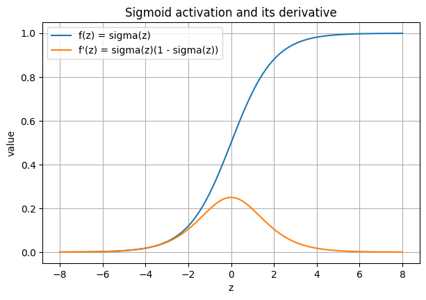
max of f'(z) is 0.25 at z = 0 (this cap matters for deep nets).
Backward pass (the error term \(\delta\) per node, right to left):
Output layer: \(\ \delta^{(n_l)} = -(y - a^{(n_l)}) \odot f'(z^{(n_l)}) = (a^{(n_l)} - y) \odot f'(z^{(n_l)})\)
Hidden layer: \(\ \delta^{(l)} = \big((W^{(l)})^{T} \delta^{(l+1)}\big) \odot f'(z^{(l)})\)
Parameter gradients (per example): \(\ \nabla_{W^{(l)}} L = \delta^{(l+1)} (a^{(l)})^{T}, \qquad \nabla_{b^{(l)}} L = \delta^{(l+1)}\)
where \(\odot\) is the elementwise (Hadamard) product. We store the \(M\) examples as
columns of \(X\) (shape (n_in, M)), so the sum over examples in
\(\nabla_{W^{(l)}} L\) becomes a single matrix product \(\delta^{(l+1)} (a^{(l)})^{T}\),
and we divide by \(M\) for the overall (averaged) cost.
def forward(X, W1, b1, W2, b2):
    "Forward pass. X has shape (n_in, M): each column is one example."
    z2 = W1 @ X + b1          # (n_hidden, M)
    a2 = sigmoid(z2)          # (n_hidden, M)
    z3 = W2 @ a2 + b2         # (n_out, M)
    a3 = sigmoid(z3)          # (n_out, M)  -> h(x), sigmoid output in (0, 1)
    return z2, a2, z3, a3

def mse_cost(a3, Y):
    "Overall cost L(theta) = (1/M) sum_i (1/2) ||a3_i - y_i||^2."
    M = Y.shape[1]
    return 0.5 * ((a3 - Y) ** 2).sum() / M

def backward(X, Y, z2, a2, z3, a3, W2):
    "Hand-derived backprop. Gradients are averaged over the M examples."
    M = X.shape[1]
    # Output error term:  delta3 = (a3 - y) . f'(z3)
    delta3 = (a3 - Y) * sigmoid_deriv(z3)
    # Hidden error term:  delta2 = (W2^T delta3) . f'(z2)
    delta2 = (W2.t() @ delta3) * sigmoid_deriv(z2)
    # Parameter gradients: grad_W = delta_{l+1} (a_l)^T, then average by 1/M.
    gW2 = (delta3 @ a2.t()) / M          # a^(2) is the input to layer 2->3
    gb2 = delta3.sum(dim=1, keepdim=True) / M
    gW1 = (delta2 @ X.t()) / M           # a^(1) = x is the input to layer 1->2
    gb1 = delta2.sum(dim=1, keepdim=True) / M
    return dict(gW1=gW1, gb1=gb1, gW2=gW2, gb2=gb2, delta2=delta2, delta3=delta3)
3. The payoff, verify against autograd#
This is the moment of truth. We build the identical
forward pass with autograd tensors, call .backward(), and compare each gradient
tensor to our hand-derived one on the same random weights and data. We work
in float64 so the agreement is essentially exact (about \(10^{-15}\)).
torch.manual_seed(1)
n0, n1, n2, M = 3, 5, 2, 4
dtype = torch.float64

# Random weights and data (the same numbers feed both methods).
vW1 = torch.randn(n1, n0, dtype=dtype, device=device)
vb1 = torch.randn(n1, 1,  dtype=dtype, device=device)
vW2 = torch.randn(n2, n1, dtype=dtype, device=device)
vb2 = torch.randn(n2, 1,  dtype=dtype, device=device)
Xv = torch.randn(n0, M, dtype=dtype, device=device)
Yv = torch.rand(n2, M,  dtype=dtype, device=device)     # targets in (0, 1)

# (a) our from-scratch gradients
z2, a2, z3, a3 = forward(Xv, vW1, vb1, vW2, vb2)
grads = backward(Xv, Yv, z2, a2, z3, a3, vW2)

# (b) autograd on an identical forward pass and the same cost
aW1 = vW1.clone().requires_grad_(True)
ab1 = vb1.clone().requires_grad_(True)
aW2 = vW2.clone().requires_grad_(True)
ab2 = vb2.clone().requires_grad_(True)
_, _, _, a3a = forward(Xv, aW1, ab1, aW2, ab2)
loss = mse_cost(a3a, Yv)
loss.backward()

pairs = [("gW1", grads["gW1"], aW1.grad), ("gb1", grads["gb1"], ab1.grad),
         ("gW2", grads["gW2"], aW2.grad), ("gb2", grads["gb2"], ab2.grad)]
max_diff = 0.0
for name, ours, auto in pairs:
    d = (ours - auto).abs().max().item()
    max_diff = max(max_diff, d)
    print("%s  max abs diff vs autograd: %.2e" % (name, d))
print("overall max abs diff:", max_diff)
assert max_diff < 1e-5, "from-scratch gradients do not match autograd!"
print("PASS: our hand-derived backprop matches autograd.")
gW1  max abs diff vs autograd: 8.67e-18
gb1  max abs diff vs autograd: 6.94e-18
gW2  max abs diff vs autograd: 1.04e-17
gb2  max abs diff vs autograd: 6.94e-18
overall max abs diff: 1.0408340855860843e-17
PASS: our hand-derived backprop matches autograd.
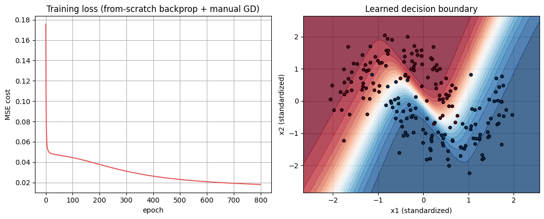
4. Train the from-scratch network with manual gradient descent#
Now we put backprop to work. Following the slide’s algorithm: for each step do a
forward pass, compute the output error, back-propagate the deltas, accumulate the
gradients over all \(M\) examples (our backward already averages), then update
every parameter with a gradient descent step
The data is sklearn.make_moons (200 points, two interleaving classes). We
standardize the inputs so the sigmoid units are not stuck in saturation.
from sklearn.datasets import make_moons

X_np, y_np = make_moons(n_samples=200, noise=0.2, random_state=0)
X_np = (X_np - X_np.mean(axis=0)) / X_np.std(axis=0)     # standardize
X_np = X_np.astype(np.float32)
y_np = y_np.astype(np.float32)

# Column layout for our from-scratch net: X is (n_features, M), Y is (1, M).
Xcol = torch.tensor(X_np.T, device=device)
Ycol = torch.tensor(y_np.reshape(1, -1), device=device)

def init_params(width=16, scale=1.0, seed=0):
    "Fresh (W1, b1, W2, b2) for a 2-input, 1-output net (reproducible)."
    g = torch.Generator(device="cpu").manual_seed(seed)
    W1 = (scale * torch.randn(width, 2, generator=g)).to(device)
    b1 = torch.zeros(width, 1, device=device)
    W2 = (scale * torch.randn(1, width, generator=g)).to(device)
    b2 = torch.zeros(1, 1, device=device)
    return W1, b1, W2, b2

def train_scratch(lr=5.0, epochs=800, width=16, scale=1.0, seed=0):
    "Manual gradient descent using our forward/backward. Returns params, losses."
    W1, b1, W2, b2 = init_params(width, scale, seed)
    losses = []
    for _ in range(epochs):
        z2, a2, z3, a3 = forward(Xcol, W1, b1, W2, b2)
        losses.append(mse_cost(a3, Ycol).item())
        g = backward(Xcol, Ycol, z2, a2, z3, a3, W2)
        W1 = W1 - lr * g["gW1"]      # theta <- theta - lr * grad
        b1 = b1 - lr * g["gb1"]
        W2 = W2 - lr * g["gW2"]
        b2 = b2 - lr * g["gb2"]
    return (W1, b1, W2, b2), losses

def accuracy(params):
    W1, b1, W2, b2 = params
    _, _, _, a3 = forward(Xcol, W1, b1, W2, b2)
    return ((a3 > 0.5).float() == Ycol).float().mean().item()

def plot_boundary(ax, params, title):
    "Contourf of the predicted probability plus the training points."
    W1, b1, W2, b2 = params
    x1 = np.linspace(X_np[:, 0].min() - 0.6, X_np[:, 0].max() + 0.6, 160)
    x2 = np.linspace(X_np[:, 1].min() - 0.6, X_np[:, 1].max() + 0.6, 160)
    xx, yy = np.meshgrid(x1, x2)
    grid = np.stack([xx.ravel(), yy.ravel()], axis=0).astype(np.float32)
    _, _, _, a3 = forward(torch.tensor(grid, device=device), W1, b1, W2, b2)
    Z = a3.detach().cpu().numpy().reshape(xx.shape)
    ax.contourf(xx, yy, Z, levels=20, cmap="RdBu", alpha=0.75)
    ax.scatter(X_np[:, 0], X_np[:, 1], c=y_np, cmap="RdBu", edgecolors="k", s=18)
    ax.set_xlabel("x1 (standardized)")
    ax.set_ylabel("x2 (standardized)")
    ax.set_title(title)
# One clean training run, then plot the loss curve and the decision boundary.
params, losses = train_scratch(lr=5.0, epochs=800)
print("final cost: %.4f    train accuracy: %.3f" % (losses[-1], accuracy(params)))

fig, (ax1, ax2) = plt.subplots(1, 2, figsize=(11, 4.5))
ax1.plot(losses, color="#e45756")
ax1.set_xlabel("epoch")
ax1.set_ylabel("MSE cost")
ax1.set_title("Training loss (from-scratch backprop + manual GD)")
plot_boundary(ax2, params, "Learned decision boundary")
plt.tight_layout()
plt.show()
final cost: 0.0181 train accuracy: 0.960
Widget: learning rate and epochs#
Retrain the from-scratch network for different learning rates and epoch counts. Too small a learning rate barely moves; a healthy value carves out the curved boundary between the two moons. Each run is a fresh network trained from the same seed, so differences come only from the hyperparameters.
def train_demo(lr=5.0, epochs=500):
    params, losses = train_scratch(lr=lr, epochs=int(epochs))
    acc = accuracy(params)
    fig, (ax1, ax2) = plt.subplots(1, 2, figsize=(11, 4.5))
    ax1.plot(losses, color="#e45756")
    ax1.set_xlabel("epoch")
    ax1.set_ylabel("MSE cost")
    ax1.set_title("Loss curve (final cost %.4f)" % losses[-1])
    plot_boundary(ax2, params, "Decision boundary (train acc %.3f)" % acc)
    plt.tight_layout()
    plt.show()

interact(train_demo,
         lr=FloatSlider(min=0.5, max=15.0, step=0.5, value=5.0),
         epochs=IntSlider(min=50, max=1500, step=50, value=500));
Widget: watch the boundary form during training#
We train once and snapshot the decision boundary at a few epochs, then let you scrub through them. Early on the boundary is nearly a straight line (the network behaves almost linearly); as training proceeds it bends to wrap the two moons.
# Pre-compute snapshots so the slider is instant.
snap_epochs = [0, 20, 60, 150, 350, 800]
sW1, sb1, sW2, sb2 = init_params(width=16, scale=1.0, seed=0)
sx1 = np.linspace(X_np[:, 0].min() - 0.6, X_np[:, 0].max() + 0.6, 140)
sx2 = np.linspace(X_np[:, 1].min() - 0.6, X_np[:, 1].max() + 0.6, 140)
sxx, syy = np.meshgrid(sx1, sx2)
sgrid = torch.tensor(np.stack([sxx.ravel(), syy.ravel()], axis=0).astype(np.float32),
                     device=device)

snapshots = []
lr_snap = 8.0
for e in range(max(snap_epochs) + 1):
    if e in snap_epochs:
        _, _, _, a3g = forward(sgrid, sW1, sb1, sW2, sb2)
        Zc = a3g.detach().cpu().numpy().reshape(sxx.shape)
        _, _, _, a3t = forward(Xcol, sW1, sb1, sW2, sb2)
        snapshots.append((e, Zc, mse_cost(a3t, Ycol).item()))
    z2, a2, z3, a3 = forward(Xcol, sW1, sb1, sW2, sb2)
    g = backward(Xcol, Ycol, z2, a2, z3, a3, sW2)
    sW1 = sW1 - lr_snap * g["gW1"]
    sb1 = sb1 - lr_snap * g["gb1"]
    sW2 = sW2 - lr_snap * g["gW2"]
    sb2 = sb2 - lr_snap * g["gb2"]

def show_snapshot(step=len(snapshots) - 1):
    e, Zc, cost_e = snapshots[int(step)]
    fig, ax = plt.subplots()
    ax.contourf(sxx, syy, Zc, levels=20, cmap="RdBu", alpha=0.75)
    ax.scatter(X_np[:, 0], X_np[:, 1], c=y_np, cmap="RdBu", edgecolors="k", s=18)
    ax.set_xlabel("x1 (standardized)")
    ax.set_ylabel("x2 (standardized)")
    ax.set_title("Boundary after %d epochs (cost %.4f)" % (e, cost_e))
    plt.show()

interact(show_snapshot,
         step=IntSlider(min=0, max=len(snapshots) - 1, step=1,
                        value=len(snapshots) - 1));
5. The same task, idiomatic PyTorch#
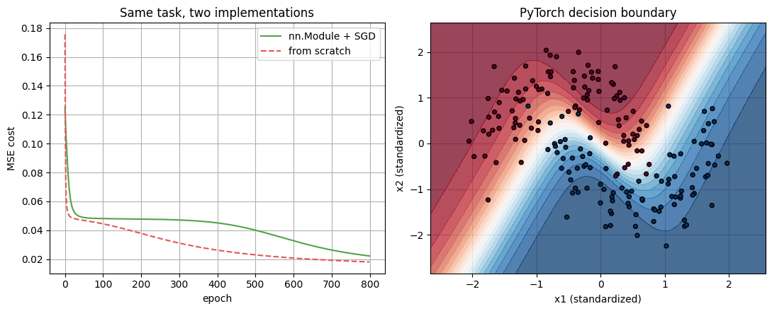
The last step: the same network the way you would actually write
it, with nn.Module, autograd, and an optimizer. It is a handful of lines and it
reaches the same accuracy and the same kind of boundary. Everything we did by
hand is exactly what these three lines (forward, loss.backward(),
optimizer.step()) do under the hood.
torch.manual_seed(0)
Xr = torch.tensor(X_np, device=device)              # (M, 2), rows are examples
Yr = torch.tensor(y_np.reshape(-1, 1), device=device)

model = nn.Sequential(
    nn.Linear(2, 16), nn.Sigmoid(),
    nn.Linear(16, 1), nn.Sigmoid(),
).to(device)
opt = torch.optim.SGD(model.parameters(), lr=5.0)
mse = nn.MSELoss()

torch_losses = []
for _ in range(800):
    opt.zero_grad()
    out = model(Xr)
    loss = 0.5 * mse(out, Yr)          # 0.5 to match our (1/2)||.||^2 cost
    loss.backward()                    # autograd does the backprop
    opt.step()                         # gradient descent update
    torch_losses.append(loss.item())

with torch.no_grad():
    acc = ((model(Xr) > 0.5).float() == Yr).float().mean().item()
print("idiomatic PyTorch  final cost: %.4f    train accuracy: %.3f" % (torch_losses[-1], acc))

# Compare loss curves and show the learned boundary.
xx, yy = np.meshgrid(
    np.linspace(X_np[:, 0].min() - 0.6, X_np[:, 0].max() + 0.6, 160),
    np.linspace(X_np[:, 1].min() - 0.6, X_np[:, 1].max() + 0.6, 160))
grid = torch.tensor(np.stack([xx.ravel(), yy.ravel()], axis=1).astype(np.float32),
                    device=device)
with torch.no_grad():
    Zt = model(grid).cpu().numpy().reshape(xx.shape)

fig, (ax1, ax2) = plt.subplots(1, 2, figsize=(11, 4.5))
ax1.plot(torch_losses, color="#54a24b", label="nn.Module + SGD")
ax1.plot(losses, color="#e45756", linestyle="--", label="from scratch")
ax1.set_xlabel("epoch")
ax1.set_ylabel("MSE cost")
ax1.set_title("Same task, two implementations")
ax1.legend()
ax2.contourf(xx, yy, Zt, levels=20, cmap="RdBu", alpha=0.75)
ax2.scatter(X_np[:, 0], X_np[:, 1], c=y_np, cmap="RdBu", edgecolors="k", s=18)
ax2.set_xlabel("x1 (standardized)")
ax2.set_ylabel("x2 (standardized)")
ax2.set_title("PyTorch decision boundary")
plt.tight_layout()
plt.show()
idiomatic PyTorch final cost: 0.0223 train accuracy: 0.950
A look ahead: where do gradients go in deep nets?#
One teaching visual to connect backprop with a problem you will meet later. Each
time a delta is passed back through a sigmoid layer it is multiplied by
\(f'(z) \le 0.25\). Stack many such layers and the gradients reaching the early
layers can become extremely small. The widget below stacks depth sigmoid layers
and plots the gradient magnitude per layer: notice the steep decay toward the
input side. This is the vanishing gradient problem, which we revisit in
Lecture 9.
def grad_per_layer(depth=5):
    torch.manual_seed(0)
    width = 8
    mods = [nn.Linear(4, width), nn.Sigmoid()]
    for _ in range(depth - 1):
        mods += [nn.Linear(width, width), nn.Sigmoid()]
    net = nn.Sequential(*mods).to(device)
    xin = torch.randn(32, 4, device=device)
    target = torch.randn(32, width, device=device)
    loss = ((net(xin) - target) ** 2).mean()
    net.zero_grad()
    loss.backward()
    norms = [m.weight.grad.norm().item() for m in net if isinstance(m, nn.Linear)]

    fig, ax = plt.subplots()
    idx = np.arange(1, len(norms) + 1)
    plot_vals = [max(v, 1e-12) for v in norms]
    ax.bar(idx, plot_vals, color="#b279a2")
    for i in range(len(norms)):
        ax.text(idx[i], plot_vals[i], "%.1e" % norms[i],
                ha="center", va="bottom", fontsize=7.5)
    ax.set_yscale("log")
    ax.set_xlabel("layer index (1 = closest to input)")
    ax.set_ylabel("gradient L2 norm (log scale)")
    ax.set_title("Per-layer weight-gradient magnitude (depth = %d)" % depth)
    plt.show()

interact(grad_per_layer, depth=IntSlider(min=2, max=8, step=1, value=5));
Key takeaways#
Backprop is the chain rule applied layer by layer, right to left, reusing the error term \(\delta\) so no derivative is computed twice.
Output error \(\delta^{(n_l)} = (a^{(n_l)} - y) \odot f'(z^{(n_l)})\); hidden error \(\delta^{(l)} = \big((W^{(l)})^{T}\delta^{(l+1)}\big) \odot f'(z^{(l)})\).
Gradients \(\nabla_{W^{(l)}} L = \delta^{(l+1)} (a^{(l)})^{T}\) and \(\nabla_{b^{(l)}} L = \delta^{(l+1)}\), averaged over the \(M\) examples.
Our hand-derived gradients matched autograd to about \(10^{-15}\): autograd is backprop, done for you.
Gradient descent then simply nudges each parameter by \(-\eta\, \nabla L\).
The sigmoid derivative caps at 0.25, so gradients can shrink through many layers (a preview of vanishing gradients).
Exercises#
Work out the tanh derivative and swap it in as the hidden activation (hint: \(\tanh'(x) = 1 - \tanh(x)^2\)). Does the boundary train faster?
Extend the from-scratch network to three weight layers (add \(W^{(3)}, b^{(3)}\)), update the backward pass, and re-verify against autograd (it should still match to about \(10^{-15}\)).