📺 Lecture video  |  📄 Slides

Watch on YouTube

Week 6, Lecture 4: CNNs for Segmentation

NPTEL Deep Learning for Computer Vision | Prof. Vineeth N Balasubramanian, IIT Hyderabad

Companion notebook for §6.3 CNNs for Segmentation.

This lecture asks “which class does every pixel belong to?”, and then “which object does every pixel belong to?”.

Contents

1. Recap of classical segmentation: Watershed, Graph Cut, Normalized Cut, Mean Shift

2. Semantic segmentation as per-pixel classification

3. FCN (Long et al, CVPR 2015): FC layers become conv layers, plus skip connections (FCN-32s / 16s / 8s)

4. Transpose convolution: learnable upsampling

5. FCN with a VGG-16 backbone

6. SegNet (Badrinarayanan et al, TPAMI 2017): unpooling with max-pool indices

7. U-Net (Ronneberger et al, MICCAI 2015): concatenation skips, elastic deformation, weighted loss

8. PSPNet (Zhao et al, CVPR 2017): the pyramid pooling module

9. DeepLab (Chen et al, TPAMI 2017): atrous / dilated convolution, ASPP, CRF

10. DeepLab v3 and v3+

11. Instance segmentation

12. Mask R-CNN (He et al, ICCV 2017): Faster R-CNN plus a mask branch

13. RoIAlign vs RoIPool

14. The FCN mask head

15. Panoptic segmentation (Kirillov et al, CVPR 2019)

16. The panoptic quality metric: \(PQ = SQ \times RQ\)

17. From metric to loss: IoU, mIoU, Dice, Dice loss

18. A taxonomy of segmentation losses

What you will learn

Everything here is built bottom-up, from scratch, and checked against PyTorch where a reference exists.

• A procedural segmentation dataset with exact semantic, instance and panoptic ground truth

• A dense prediction head, by deleting the global average pool from a classifier (and proving the two are the same layer)

• Transpose convolution from scratch, in 1D and 2D, verified with assert torch.allclose(...) against nn.ConvTranspose1d / nn.ConvTranspose2d

• The checkerboard artifact, and the rule that avoids it

• SegNet unpooling that reproduces the exact figure from the lecture slides

• A tiny U-Net, block by block, trained on CPU, plus a real measured skip-connection ablation

• Dilated convolution receptive fields, measured with autograd, and a mini ASPP

• A mini pyramid pooling module

• RoIPool and RoIAlign from scratch, cross-checked against torchvision.ops, and a demo of why quantization breaks masks

• IoU, mIoU, Dice, Dice loss and Panoptic Quality from scratch, with \(PQ = SQ \times RQ\) verified numerically

• Eight interactive sliders to build intuition

How to run

Runs top to bottom on Google Colab CPU in roughly 3 minutes (faster on GPU). No downloads, no pretrained weights, no pip install. Only torch, torchvision, numpy, matplotlib, scipy and ipywidgets.

Review

Lectures 1 to 3 of this week asked “where are the objects?” and answered with boxes.

Setup

• One cell of imports, one random seed, one device. %matplotlib inline is what makes the sliders render in Colab.

• Everything is written to work on CPU. If a GPU happens to be present it is used, but nothing here needs one.

%matplotlib inline
import time, math
import numpy as np
import torch
import torch.nn as nn
import torch.nn.functional as F
import torchvision
import matplotlib.pyplot as plt
import matplotlib.patches as mpatches
import scipy.ndimage as ndi
import ipywidgets as widgets
from IPython.display import display

SEED = 0

def set_seed(s=SEED):
    np.random.seed(s)
    torch.manual_seed(s)

set_seed()
device = torch.device('cuda' if torch.cuda.is_available() else 'cpu')
torch.set_num_threads(min(4, torch.get_num_threads()))     # keep CPU runtime predictable on Colab

plt.rcParams.update({'figure.dpi': 110, 'axes.grid': False, 'image.interpolation': 'nearest',
                     'axes.titlesize': 9, 'axes.labelsize': 8,
                     'xtick.labelsize': 7, 'ytick.labelsize': 7, 'legend.fontsize': 8})

print('torch      :', torch.__version__)
print('torchvision:', torchvision.__version__)
print('device     :', device)

torch      : 2.8.0
torchvision: 0.23.0
device     : cpu

0. A synthetic dataset with semantic, instance and panoptic ground truth

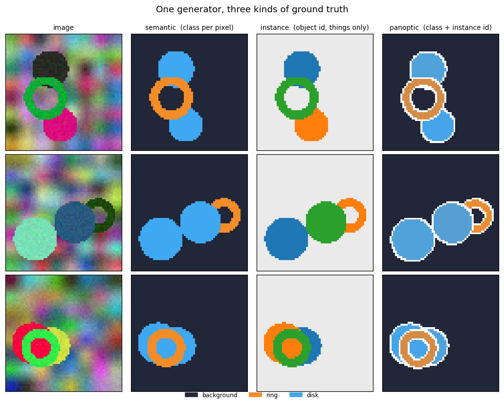
Segmentation labels are expensive: every pixel needs a category. The slides call this “quite annotation-intensive”, and that is the practical reason segmentation datasets are smaller than classification datasets. We sidestep it by generating our data, which also gives us perfect ground truth for free.

Each \(64 \times 64\) image contains:

• a textured background: a low-frequency random colour field, faint stripes and grain (this is “stuff”)

• 3 or 4 shapes drawn on top of it, in occlusion order (these are “things”):

  • class 1 = ring: an annulus, 4 to 5 pixels thick, with a hole in the middle (a thin structure)

  • class 2 = disk: a solid filled circle

Three design decisions that matter for the rest of the notebook:

• Colour carries no class information. Each shape’s colour is drawn uniformly at random and is only rejected if it fails to contrast with the local background. The background contains every hue too. So a per-pixel colour lookup cannot solve this task: the network must use spatial context to decide what is an object and which class it is.

• The class is decidable locally, but the boundary is not. Ring versus disk is “is there a hole?”, answerable in a small neighbourhood, so the classifier trains fast and reliably. But the ring is a thin structure: a decoder that only sees the coarse \(8 \times 8\) bottleneck cannot reconstruct its hole or its two edges. That is exactly what makes the U-Net skip ablation later a real experiment rather than a slogan.

• Rings are on-theme. U-Net was designed for biomedical images full of thin structures (cell membranes, vessels), where getting the boundary right is the whole game.

Three labels come out of the same generator:

Label	Meaning	Shape
sem	semantic class id per pixel, in \(\{0, 1, 2\}\)	(H, W)
inst	instance id per pixel, 0 for background, 1..K for things	(H, W)
panoptic	the pair (sem, inst) per pixel	derived

IMG = 64
NUM_CLASSES = 3                                  # background + 2 thing classes  (this is the "C + 1" of the slides)
CLASS_NAMES = ['background', 'ring', 'disk']
CLASS_COLORS = np.array([[0.13, 0.15, 0.22],     # background (stuff)
                         [0.96, 0.55, 0.16],     # ring       (thing)
                         [0.25, 0.66, 0.95]])    # disk       (thing)
THING_CLASSES = [1, 2]                            # classes that have instances
STUFF_CLASSES = [0]

def _background(rng, H, W):
    """Low-frequency random colour field + faint stripes + grain."""
    small = rng.uniform(0.15, 0.85, size=(1, 3, 8, 8)).astype(np.float32)
    bg = F.interpolate(torch.from_numpy(small), size=(H, W), mode='bilinear', align_corners=False)[0].numpy()
    yy = np.arange(H, dtype=np.float32)[None, :, None]
    xx = np.arange(W, dtype=np.float32)[None, None, :]
    bg = bg + 0.06 * np.sin(yy / rng.uniform(2.0, 4.0) + rng.uniform(0, 6.28))
    bg = bg + 0.04 * np.sin(xx / rng.uniform(2.0, 5.0) + rng.uniform(0, 6.28))
    bg = bg + rng.normal(0, 0.03, size=bg.shape).astype(np.float32)
    return np.clip(bg, 0, 1).astype(np.float32)

def shape_mask(kind, cy, cx, r, thick, yy, xx):
    """kind 0 -> ring (annulus of thickness `thick`), kind 1 -> disk (solid). Boolean mask."""
    d = np.sqrt((yy - cy) ** 2 + (xx - cx) ** 2)
    if kind == 0:
        return (d <= r) & (d >= r - thick)
    return d <= r

def make_sample(rng, H=IMG, W=IMG, n_range=(3, 4)):
    """Returns img (3,H,W) float32 in [0,1], sem (H,W) int64, inst (H,W) int64."""
    img = _background(rng, H, W)
    sem = np.zeros((H, W), np.int64)
    inst = np.zeros((H, W), np.int64)
    yy, xx = np.mgrid[0:H, 0:W].astype(np.float32)
    for k in range(int(rng.integers(n_range[0], n_range[1] + 1))):
        kind = int(rng.integers(0, 2))
        r = rng.uniform(9.0, 13.0)
        thick = rng.uniform(4.0, 5.0)
        cy, cx = rng.uniform(r + 2, H - r - 2), rng.uniform(r + 2, W - r - 2)
        m = shape_mask(kind, cy, cx, r, thick, yy, xx)
        if m.sum() < 15:
            continue
        # pick a colour that is uninformative about the class but contrasts with the local background
        local = img[:, m].mean(axis=1)
        color = np.clip(1.0 - local, 0, 1)
        for _ in range(30):
            c = rng.uniform(0, 1, size=3).astype(np.float32)
            if np.linalg.norm(c - local) > 0.45:
                color = c
                break
        img[:, m] = color[:, None] + rng.normal(0, 0.03, size=(3, int(m.sum()))).astype(np.float32)
        sem[m] = kind + 1          # later shapes occlude earlier ones
        inst[m] = k + 1
    # occlusion can wipe an instance out entirely: relabel the survivors 1..K
    out_inst = np.zeros_like(inst)
    for new_id, old_id in enumerate([v for v in np.unique(inst) if v != 0], start=1):
        out_inst[inst == old_id] = new_id
    return np.clip(img, 0, 1).astype(np.float32), sem, out_inst

def make_dataset(n, seed, **kw):
    rng = np.random.default_rng(seed)
    X, S, I = [], [], []
    for _ in range(n):
        img, sem, inst = make_sample(rng, **kw)
        X.append(img); S.append(sem); I.append(inst)
    return (torch.from_numpy(np.stack(X)), torch.from_numpy(np.stack(S)), torch.from_numpy(np.stack(I)))

t0 = time.time()
Xtr, Str, Itr = make_dataset(256, seed=0)     # "very few training images", in the spirit of the U-Net paper
Xva, Sva, Iva = make_dataset(64, seed=1)
print(f'generated train {tuple(Xtr.shape)} and val {tuple(Xva.shape)} in {time.time()-t0:.2f} s')
print('\nclass pixel frequencies (train):')
for c in range(NUM_CLASSES):
    print(f'  {c}  {CLASS_NAMES[c]:11s} {(Str == c).float().mean():.3f}')
print(f'\nmean instances per image: {np.mean([Itr[i].max().item() for i in range(len(Itr))]):.2f}')

generated train (256, 3, 64, 64) and val (64, 3, 64, 64) in 0.12 s

class pixel frequencies (train):
  0  background  0.779
  1  ring        0.086
  2  disk        0.135

mean instances per image: 3.44

The same image, three ways

This single figure is the map for the whole lecture:

• semantic: every pixel gets a class. Two overlapping disks are one blue region. This is sections 2 to 10.

• instance: every thing pixel gets an object id. Background is not labelled at all. This is sections 11 to 14.

• panoptic: every pixel gets a class and, if it is a thing, an instance id. This is sections 15 to 16.

In the panoptic panel the fill colour is the class and the white contours separate instances.

INST_COLORS = np.array(plt.get_cmap('tab10').colors)

def semantic_rgb(sem):
    return CLASS_COLORS[sem]

def instance_rgb(inst):
    out = np.full(inst.shape + (3,), 0.92)                      # unlabelled = light grey
    for k in range(1, int(inst.max()) + 1):
        out[inst == k] = INST_COLORS[(k - 1) % len(INST_COLORS)]
    return out

def instance_contours(inst):
    b = np.zeros(inst.shape, bool)
    b[1:, :] |= inst[1:, :] != inst[:-1, :]
    b[:, 1:] |= inst[:, 1:] != inst[:, :-1]
    return b

def panoptic_rgb(sem, inst):
    """Class colour as the fill, a deterministic per-instance shade, white contours to separate objects."""
    out = CLASS_COLORS[sem].copy()
    for k in range(1, int(inst.max()) + 1):
        m = inst == k
        f = 0.65 + 0.35 * ((0.37 * k) % 1.0)
        out[m] = np.clip(out[m] * f + (1 - f) * 0.55, 0, 1)
    out[instance_contours(inst)] = 1.0
    return out

def show_row(axes, img, sem, inst, titles=True):
    axes[0].imshow(img.transpose(1, 2, 0))
    axes[1].imshow(semantic_rgb(sem))
    axes[2].imshow(instance_rgb(inst))
    axes[3].imshow(panoptic_rgb(sem, inst))
    if titles:
        for ax, t in zip(axes, ['image', 'semantic  (class per pixel)',
                                'instance  (object id, things only)',
                                'panoptic  (class + instance id)']):
            ax.set_title(t)
    for ax in axes:
        ax.set_xticks([]); ax.set_yticks([])

fig, axes = plt.subplots(3, 4, figsize=(9.5, 7.4))
for r in range(3):
    show_row(axes[r], Xva[r].numpy(), Sva[r].numpy(), Iva[r].numpy(), titles=(r == 0))
handles = [mpatches.Patch(color=CLASS_COLORS[c], label=CLASS_NAMES[c]) for c in range(NUM_CLASSES)]
fig.legend(handles=handles, loc='lower center', ncol=3, frameon=False, bbox_to_anchor=(0.5, -0.01))
fig.suptitle('One generator, three kinds of ground truth', y=0.99)
plt.tight_layout(); plt.show()

1. Recap: classical image segmentation

Before deep learning, segmentation meant grouping pixels by low-level affinity. The lecture names four families:

Method	Idea in one line	Grouping criterion
Watershed	Treat intensity as a landscape, flood it from local minima, build dams where basins meet	catchment basins of the gradient
Graph Cut	Pixels are graph nodes, edges weigh similarity, cut the graph at minimum cost	min cut / max flow
Normalized Cut	Min cut is biased toward slicing off tiny regions, so normalize the cut by region volume	eigenvectors of a normalized affinity matrix
Mean Shift	Every pixel climbs to a mode of the feature-space density; one mode = one region	modes of a kernel density estimate

Why they matter for this course:

• They inspired the early deep detectors. R-CNN had a variant that used CPMC (Constrained Parametric Min-Cuts), a min-cut segmentation method, to propose foreground segments instead of using Selective Search boxes.

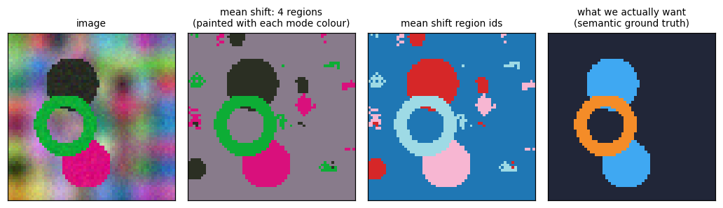
• They are unsupervised: they partition an image into regions, but they cannot name a region. There is no “ring” and no “disk” in the output, and no notion of a second disk.

That gap is exactly what the rest of this lecture fills. Let us make it concrete by running one of them.

Mean Shift, from scratch, on our image

• Treat each pixel’s RGB as a point in a 3D feature space.

• Every point repeatedly moves to the Gaussian-weighted mean of its neighbours: \(\; x \leftarrow \frac{\sum_j K(x - x_j)\, x_j}{\sum_j K(x - x_j)}\).

• Points that converge to the same mode form a region.

• We run it on a random subsample of pixels (mean shift is \(O(N^2)\) per iteration) and then assign every pixel to the nearest mode.

def mean_shift(X, bandwidth=0.12, iters=12):
    """X: (N, d) points. Returns the converged position of each point."""
    P = X.copy()
    for _ in range(iters):
        d2 = ((P[:, None, :] - X[None, :, :]) ** 2).sum(-1)      # (N, N)
        w = np.exp(-d2 / (2 * bandwidth ** 2))
        with np.errstate(divide='ignore', over='ignore', invalid='ignore'):
            # some BLAS backends raise a spurious FPE flag on this float matmul; the result is finite and correct
            P = (w @ X) / np.maximum(w.sum(1, keepdims=True), 1e-12)
    return P

def mean_shift_segment(img, bandwidth=0.12, n_sub=500, seed=0):
    rng = np.random.default_rng(seed)
    feats = img.reshape(3, -1).T                                  # (H*W, 3) RGB only
    sub = feats[rng.choice(len(feats), n_sub, replace=False)]
    modes = mean_shift(sub, bandwidth)
    centers = []                                                  # merge modes closer than bandwidth/2
    for m in modes:
        if not any(np.linalg.norm(m - c) < bandwidth / 2 for c in centers):
            centers.append(m)
    centers = np.stack(centers)
    lab = np.argmin(((feats[:, None, :] - centers[None]) ** 2).sum(-1), axis=1)
    return lab.reshape(img.shape[1:]), centers

img = Xva[0].numpy()
t0 = time.time()
ms_lab, centers = mean_shift_segment(img)
print(f'mean shift found {len(centers)} modes in {time.time()-t0:.2f} s')

fig, axes = plt.subplots(1, 4, figsize=(9.5, 2.6))
axes[0].imshow(img.transpose(1, 2, 0)); axes[0].set_title('image')
axes[1].imshow(centers[ms_lab]); axes[1].set_title(f'mean shift: {len(centers)} regions\n(painted with each mode colour)')
axes[2].imshow(ms_lab, cmap='tab20'); axes[2].set_title('mean shift region ids')
axes[3].imshow(semantic_rgb(Sva[0].numpy())); axes[3].set_title('what we actually want\n(semantic ground truth)')
for ax in axes:
    ax.set_xticks([]); ax.set_yticks([])
plt.tight_layout(); plt.show()

print('Mean shift did partition the image, but notice what it cannot do:')
print('  - it splits the smooth background into several bands (different colours -> different modes)')
print('  - it merges a ring and a disk if they happen to share a colour')
print('  - the region ids are arbitrary: nothing says "this region is a ring"')
print('  - it never saw a label, so it has no way to learn what a "ring" is')

mean shift found 4 modes in 0.04 s
Mean shift did partition the image, but notice what it cannot do:
  - it splits the smooth background into several bands (different colours -> different modes)
  - it merges a ring and a disk if they happen to share a colour
  - the region ids are arbitrary: nothing says "this region is a ring"
  - it never saw a label, so it has no way to learn what a "ring" is

2. Semantic segmentation = per-pixel classification

The slides put it in one line:

Task of grouping together similar (in semantic content) pixels in an image. How to formulate this using DNNs? Cast as a pixel classification problem!

So the target is no longer one label per image, it is an \(H \times W\) grid of labels, and the network output is \((N, C+1, H, W)\) class scores, trained with the sum of pixel-wise cross-entropy losses:

\[\mathcal{L} = \frac{1}{HW}\sum_{i=1}^{H}\sum_{j=1}^{W} -\log \frac{\exp(z_{ij, y_{ij}})}{\sum_{c} \exp(z_{ij, c})}\]

2a. A classifier already contains a segmentation head

Here is the observation the whole of FCN rests on. Take any classification CNN:

• conv trunk produces a feature map of shape \((N, C_{\text{feat}}, h, w)\)

• global average pool collapses it to \((N, C_{\text{feat}})\)

• linear layer maps it to \((N, K)\) class scores

The pool is the only thing that destroys the spatial dimensions. Delete it, turn the linear layer into a \(1 \times 1\) convolution, and the same weights now emit a class score at every spatial position.

Let us verify that claim rather than assert it: with the weights copied across, a \(1\times1\) conv followed by a global average pool is identical to a global average pool followed by a linear layer (averaging and a linear map commute).

class TinyTrunk(nn.Module):
    """A small conv trunk. Two stride-2 pools -> total stride 4."""
    def __init__(self, cout=32):
        super().__init__()
        self.net = nn.Sequential(
            nn.Conv2d(3, 16, 3, padding=1), nn.ReLU(),
            nn.MaxPool2d(2),                                   # stride 2
            nn.Conv2d(16, cout, 3, padding=1), nn.ReLU(),
            nn.MaxPool2d(2),                                   # stride 4
            nn.Conv2d(cout, cout, 3, padding=1), nn.ReLU())
    def forward(self, x):
        return self.net(x)

set_seed()
trunk = TinyTrunk()
x = Xva[:4]
feat = trunk(x)
print(f'input          {tuple(x.shape)}')
print(f'trunk features {tuple(feat.shape)}   <- spatial size divided by 4 by the two pools')

# (a) the classification head: pool away all spatial information, then classify
gap_head = nn.Linear(32, NUM_CLASSES)
logits_image = gap_head(feat.mean(dim=(2, 3)))
print(f'\n(a) GAP + Linear  -> {tuple(logits_image.shape)}   ONE label for the whole image')

# (b) the dense head: the SAME layer, applied at every position, as a 1x1 convolution
dense_head = nn.Conv2d(32, NUM_CLASSES, kernel_size=1)
dense_head.weight.data = gap_head.weight.data.view(NUM_CLASSES, 32, 1, 1).clone()
dense_head.bias.data = gap_head.bias.data.clone()
logits_map = dense_head(feat)
print(f'(b) 1x1 Conv2d    -> {tuple(logits_map.shape)}   a label for EVERY position')

# the two heads are the same layer: pooling and a linear map commute
assert torch.allclose(logits_image, logits_map.mean(dim=(2, 3)), atol=1e-5)
print('\nassert torch.allclose(GAP -> Linear,  1x1 Conv -> GAP)   PASSED')
print('  => a classification head IS a dense head with a global average pool bolted on the end.')
print('  => remove the pool and you have a segmentation network. Everything else is a resolution problem.')

input          (4, 3, 64, 64)
trunk features (4, 32, 16, 16)   <- spatial size divided by 4 by the two pools

(a) GAP + Linear  -> (4, 3)   ONE label for the whole image
(b) 1x1 Conv2d    -> (4, 3, 16, 16)   a label for EVERY position

assert torch.allclose(GAP -> Linear,  1x1 Conv -> GAP)   PASSED
  => a classification head IS a dense head with a global average pool bolted on the end.
  => remove the pool and you have a segmentation network. Everything else is a resolution problem.

2b. The resolution problem, seen immediately

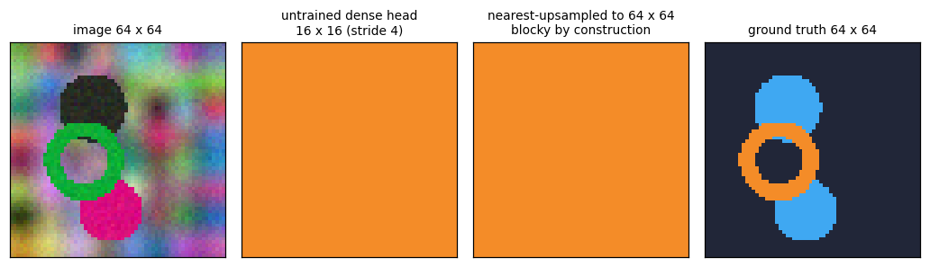
The dense head gives us a prediction per feature map cell, not per pixel. Our trunk has stride 4, so a \(64 \times 64\) image yields a \(16 \times 16\) label map. Blow it back up with nearest-neighbour and the problem is obvious: the prediction is quantised to a 4-pixel grid before it is even trained.

Real classifiers are far worse: VGG-16 has stride 32. A \(224 \times 224\) image becomes a \(7 \times 7\) score map.

pred_map = logits_map.argmax(1)                                   # (4, 16, 16)
up_nearest = F.interpolate(pred_map[:, None].float(), size=(64, 64), mode='nearest')[:, 0].long()

fig, axes = plt.subplots(1, 4, figsize=(9.5, 2.6))
axes[0].imshow(Xva[0].numpy().transpose(1, 2, 0)); axes[0].set_title('image 64 x 64')
axes[1].imshow(semantic_rgb(pred_map[0].numpy())); axes[1].set_title('untrained dense head\n16 x 16 (stride 4)')
axes[2].imshow(semantic_rgb(up_nearest[0].numpy())); axes[2].set_title('nearest-upsampled to 64 x 64\nblocky by construction')
axes[3].imshow(semantic_rgb(Sva[0].numpy())); axes[3].set_title('ground truth 64 x 64')
for ax in axes:
    ax.set_xticks([]); ax.set_yticks([])
plt.tight_layout(); plt.show()

print('Output stride of some standard classification backbones:')
for name, s in [('LeNet-ish (our trunk)', 4), ('AlexNet', 32), ('VGG-16', 32), ('ResNet-50', 32), ('GoogLeNet', 32)]:
    print(f'  {name:22s} stride {s:2d}  ->  a 224 x 224 image gives a {224//s} x {224//s} score map')

Output stride of some standard classification backbones:
  LeNet-ish (our trunk)  stride  4  ->  a 224 x 224 image gives a 56 x 56 score map
  AlexNet                stride 32  ->  a 224 x 224 image gives a 7 x 7 score map
  VGG-16                 stride 32  ->  a 224 x 224 image gives a 7 x 7 score map
  ResNet-50              stride 32  ->  a 224 x 224 image gives a 7 x 7 score map
  GoogLeNet              stride 32  ->  a 224 x 224 image gives a 7 x 7 score map

3. Fully Convolutional Networks (FCN)

Long et al, CVPR 2015 (the journal version, Shelhamer et al TPAMI 2016, is the one cited on the slide).

The recipe:

• Take a classification net (VGG-16, GoogLeNet).

• Convert its FC layers into conv layers. This is not an approximation, it is an exact re-parameterisation.

• Append a \(1 \times 1\) conv with \(C+1\) channels to produce per-pixel class scores (\(C\) classes plus background).

• The net now has lower resolution than the input, because of the max-pools. So upsample back, with a learnable transpose convolution.

• Fuse coarse, deep layers with fine, shallow layers using skip connections: FCN-32s, FCN-16s, FCN-8s.

3a. An FC layer is a convolution

The trick is pure index bookkeeping:

• A linear layer on a flattened \((C, h, w)\) feature map has weight \((K,\, C\!\cdot\!h\!\cdot\!w)\).

• x.flatten(1) lays the map out in the order \(c\), then \(i\), then \(j\). So reshaping the weight to \((K, C, h, w)\) gives exactly a conv kernel of size \(h \times w\).

• Later FC layers act on \(1 \times 1\) maps, so they become \(1 \times 1\) convs. This is the “converting FC layers into \(1\times1\) conv layers” of the slide. (In VGG-16, fc6 becomes a \(7\times7\) conv because pool5 is \(7 \times 7\); fc7 and fc8 become \(1 \times 1\) convs.)

Why bother? Because a conv does not care about its input size. The FC classifier only accepts one input size. The convolutional twin accepts any size and returns a map of classifications, computing the whole sliding window in one pass with shared computation.

set_seed()
C, h, w = 32, 4, 4
feat = torch.randn(2, C, h, w)

# --- an ordinary FC classifier head: flatten -> fc6 -> fc7 -> fc8 ---
fc6 = nn.Linear(C * h * w, 64)
fc7 = nn.Linear(64, 64)
fc8 = nn.Linear(64, NUM_CLASSES)
def head_fc(f):
    return fc8(F.relu(fc7(F.relu(fc6(f.flatten(1))))))

# --- its fully-convolutional twin: fc6 -> (h x w) conv,  fc7/fc8 -> 1x1 convs ---
c6 = nn.Conv2d(C, 64, kernel_size=(h, w))
c7 = nn.Conv2d(64, 64, kernel_size=1)
c8 = nn.Conv2d(64, NUM_CLASSES, kernel_size=1)
c6.weight.data = fc6.weight.data.view(64, C, h, w).clone(); c6.bias.data = fc6.bias.data.clone()
c7.weight.data = fc7.weight.data.view(64, 64, 1, 1).clone(); c7.bias.data = fc7.bias.data.clone()
c8.weight.data = fc8.weight.data.view(NUM_CLASSES, 64, 1, 1).clone(); c8.bias.data = fc8.bias.data.clone()
def head_conv(f):
    return c8(F.relu(c7(F.relu(c6(f)))))

a, b = head_fc(feat), head_conv(feat)
print(f'FC head            {tuple(a.shape)}')
print(f'conv head          {tuple(b.shape)}  -> squeeze the 1x1 spatial dims -> {tuple(b.flatten(1).shape)}')
assert torch.allclose(a, b.flatten(1), atol=1e-5)
print(f'max |difference| = {(a - b.flatten(1)).abs().max():.2e}')
print('assert torch.allclose(FC head, conv head)   PASSED  -> same function, same parameters\n')

# --- the payoff: feed a LARGER map. The FC head cannot. The conv head returns a score MAP. ---
big = torch.randn(1, C, 12, 12)
out_big = head_conv(big)
print(f'conv head on a {tuple(big.shape[2:])} feature map -> {tuple(out_big.shape)}')
print(f'  that is {out_big.shape[2]} x {out_big.shape[3]} = {out_big.shape[2]*out_big.shape[3]} classifications, '
      f'one per sliding-window position, in a single pass with shared work.')
try:
    head_fc(big)
except RuntimeError as e:
    print(f'\nthe FC head on the same input raises:\n  RuntimeError: {str(e)[:96]}...')

FC head            (2, 3)
conv head          (2, 3, 1, 1)  -> squeeze the 1x1 spatial dims -> (2, 3)
max |difference| = 2.98e-08
assert torch.allclose(FC head, conv head)   PASSED  -> same function, same parameters

conv head on a (12, 12) feature map -> (1, 3, 9, 9)
  that is 9 x 9 = 81 classifications, one per sliding-window position, in a single pass with shared work.

the FC head on the same input raises:
  RuntimeError: mat1 and mat2 shapes cannot be multiplied (1x4608 and 512x64)...

4. Transpose convolution: learnable upsampling

The slide lists the names you will meet in papers, and its opinion of one of them:

• Transpose convolution (the accurate name: it is the transpose of the matrix a convolution multiplies by)

• Deconvolution (marked “bad” on the slide, and rightly: it does not invert a convolution)

• Upconvolution

• Fractionally strided convolution (a stride-\(s\) transpose conv slides the kernel by \(1/s\) of an output step)

The motivation is one question:

Traditionally, we could achieve upsampling through interpolation or similar rules. Why not allow the network to learn the rules by itself?

Bilinear interpolation applies the same fixed averaging rule to a mask boundary and to a flat interior region. A transpose conv has weights, so it can learn a rule that sharpens boundaries instead of blurring them.

The mechanics

A normal convolution takes a window of inputs and produces one output: many to one. A transpose convolution does the adjoint: it takes one input and scatters a scaled copy of the kernel into a window of outputs: one to many. Overlapping copies are summed.

Output size, for input size \(i\), kernel \(k\), stride \(s\), padding \(p\):

\[o = s\,(i - 1) + k - 2p\]

Note that padding crops the output here, which is the opposite of what it does in a normal convolution. That is the tell-tale sign that this is a transpose: every argument plays the role it would play in the forward conv whose gradient this is.

4a. The 1D case, from scratch

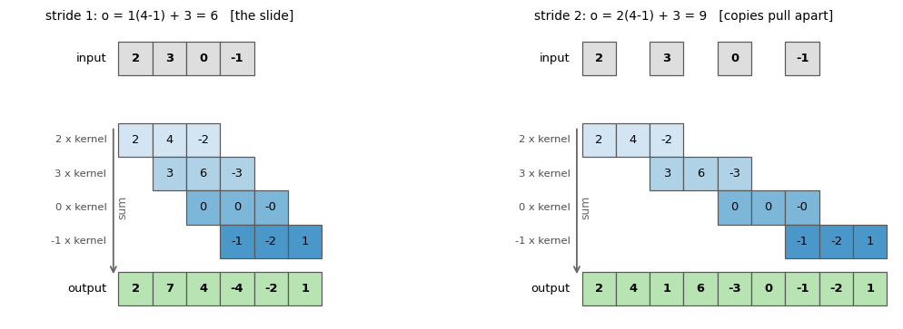
We implement exactly the example on the slide: input \([2, 3, 0, -1]\), kernel \([1, 2, -1]\), \(s=1\), \(p=0\).

• Each input value scales the whole kernel, the copy is dropped at offset \(i \cdot s\), and the copies are summed.

• Output length \(= W + w - 1 = 4 + 3 - 1 = 6\), which is the formula above with \(s=1, p=0\).

• We then check the from-scratch version against nn.ConvTranspose1d on random multi-channel tensors with random stride and padding, because matching one hand-picked example is not evidence.

def conv_transpose1d_scratch(x, w, b=None, stride=1, padding=0):
    """x: (Cin, L). w: (Cin, Cout, K) -- PyTorch's transpose-conv weight layout. Returns (Cout, L_out)."""
    Cin, L = x.shape
    _, Cout, K = w.shape
    full = np.zeros((Cout, stride * (L - 1) + K))
    for i in range(L):                                  # scatter: one input -> many outputs
        full[:, i * stride: i * stride + K] += np.tensordot(x[:, i], w, axes=([0], [0]))
    if padding:                                         # padding CROPS the output
        full = full[:, padding: full.shape[1] - padding]
    return full + (b[:, None] if b is not None else 0.0)

# ---- the exact example from the slide ----
x_slide = np.array([[2.0, 3.0, 0.0, -1.0]])
w_slide = np.array([[[1.0, 2.0, -1.0]]])
out_scratch = conv_transpose1d_scratch(x_slide, w_slide)
out_torch = F.conv_transpose1d(torch.tensor(x_slide)[None], torch.tensor(w_slide))[0].numpy()

print('input  :', x_slide[0].tolist())
print('kernel :', w_slide[0, 0].tolist())
print('scratch:', out_scratch[0].tolist())
print('pytorch:', out_torch[0].tolist())
assert np.allclose(out_scratch, out_torch)
assert np.allclose(out_scratch[0], [2, 7, 4, -4, -2, 1])
print('matches the slide, and matches nn.ConvTranspose1d\n')

# ---- the real test: random channels, random stride, random padding ----
set_seed()
for (Cin, Cout, K, s, p, L) in [(1, 1, 3, 1, 0, 4), (2, 3, 4, 2, 1, 5), (3, 2, 5, 3, 2, 4), (4, 4, 2, 2, 0, 6)]:
    xr = np.random.randn(Cin, L)
    wr = np.random.randn(Cin, Cout, K)
    br = np.random.randn(Cout)
    got = conv_transpose1d_scratch(xr, wr, br, s, p)
    ref = F.conv_transpose1d(torch.tensor(xr)[None], torch.tensor(wr), torch.tensor(br),
                             stride=s, padding=p)[0].numpy()
    assert np.allclose(got, ref), (Cin, Cout, K, s, p)
    print(f'Cin={Cin} Cout={Cout} K={K} s={s} p={p} | L={L} -> L_out={got.shape[1]:2d} '
          f'| formula s(i-1)+k-2p = {s*(L-1)+K-2*p:2d} | max|diff| vs PyTorch = {np.abs(got-ref).max():.2e}')
print('\nassert np.allclose(scratch, nn.ConvTranspose1d)   PASSED for all cases')

input  : [2.0, 3.0, 0.0, -1.0]
kernel : [1.0, 2.0, -1.0]
scratch: [2.0, 7.0, 4.0, -4.0, -2.0, 1.0]
pytorch: [2.0, 7.0, 4.0, -4.0, -2.0, 1.0]
matches the slide, and matches nn.ConvTranspose1d

Cin=1 Cout=1 K=3 s=1 p=0 | L=4 -> L_out= 6 | formula s(i-1)+k-2p =  6 | max|diff| vs PyTorch = 0.00e+00
Cin=2 Cout=3 K=4 s=2 p=1 | L=5 -> L_out=10 | formula s(i-1)+k-2p = 10 | max|diff| vs PyTorch = 8.88e-16
Cin=3 Cout=2 K=5 s=3 p=2 | L=4 -> L_out=10 | formula s(i-1)+k-2p = 10 | max|diff| vs PyTorch = 4.44e-16
Cin=4 Cout=4 K=2 s=2 p=0 | L=6 -> L_out=12 | formula s(i-1)+k-2p = 12 | max|diff| vs PyTorch = 4.44e-16

assert np.allclose(scratch, nn.ConvTranspose1d)   PASSED for all cases

4b. Watching the copies land

The figure below is the slide’s diagram, drawn from our own numbers:

• one row per input value, showing that value’s scaled copy of the kernel, dropped at offset \(i \cdot s\)

• the bottom row is the sum of the columns, which is the output

• change stride to 2 and watch the copies pull apart and the output stretch

def draw_transpose1d(x, w, stride=1, ax=None, title=None):
    x, w = np.asarray(x, float), np.asarray(w, float)
    L, K = len(x), len(w)
    Lout = stride * (L - 1) + K
    rows = np.zeros((L, Lout))
    for i in range(L):
        rows[i, i * stride:i * stride + K] = x[i] * w
    out = rows.sum(0)
    if ax is None:
        _, ax = plt.subplots(figsize=(0.78 * Lout + 1.6, 0.62 * (L + 2.4)))
    def cell(c, r, val, face, bold=False):
        ax.add_patch(mpatches.Rectangle((c, r), 1, 1, facecolor=face, edgecolor='0.35', lw=0.8))
        ax.text(c + 0.5, r + 0.5, f'{val:g}', ha='center', va='center', fontsize=8.5,
                fontweight='bold' if bold else 'normal')
    for i in range(L):                                                   # input row
        cell(i * stride, L + 1.4, x[i], '0.87', bold=True)
    ax.text(-0.35, L + 1.9, 'input', ha='right', va='center', fontsize=8.5)
    for i in range(L):                                                   # contribution rows
        r = L - 1 - i
        for j in range(K):
            cell(i * stride + j, r, rows[i, i * stride + j], plt.get_cmap('Blues')(0.18 + 0.14 * i))
        ax.text(-0.35, r + 0.5, f'{x[i]:g} x kernel', ha='right', va='center', fontsize=7.5, color='0.3')
    for c in range(Lout):                                                # output row
        cell(c, -1.4, out[c], plt.get_cmap('Greens')(0.30), bold=True)
    ax.text(-0.35, -0.9, 'output', ha='right', va='center', fontsize=8.5)
    ax.annotate('', xy=(-0.15, -0.55), xytext=(-0.15, L - 0.1),
                arrowprops=dict(arrowstyle='->', color='0.4', lw=1.2))
    ax.text(-0.05, L / 2 - 0.5, 'sum', fontsize=8, color='0.4', rotation=90, va='center')
    ax.set_xlim(-3.2, Lout + 0.2); ax.set_ylim(-1.8, L + 2.8)
    ax.set_aspect('equal'); ax.axis('off')
    ax.set_title(title or f'kernel {w.tolist()},  stride {stride}  ->  output length {Lout}')
    return out

fig, axes = plt.subplots(1, 2, figsize=(11, 3.4))
draw_transpose1d([2, 3, 0, -1], [1, 2, -1], stride=1, ax=axes[0],
                 title='stride 1: o = 1(4-1) + 3 = 6   [the slide]')
draw_transpose1d([2, 3, 0, -1], [1, 2, -1], stride=2, ax=axes[1],
                 title='stride 2: o = 2(4-1) + 3 = 9   [copies pull apart]')
plt.tight_layout(); plt.show()
print('The output is a sum of scaled, shifted copies of the kernel. The stride sets how far apart they land.')

The output is a sum of scaled, shifted copies of the kernel. The stride sets how far apart they land.

4c. The 2D case: \(2 \times 2 \to 5 \times 5\)

This is the Dumoulin figure on the slide. Reading off the picture: a \(2 \times 2\) input, a \(3 \times 3\) kernel, stride 2, padding 0, giving

\[o = s(i-1) + k - 2p = 2(2-1) + 3 - 0 = 5\]

It is the transpose of convolving a \(3\times3\) kernel over a \(5\times5\) input with stride 2 and no padding (which maps \(5 \times 5 \to 2 \times 2\)). That is where the name comes from: the two operations have transposed shapes, and each is the gradient of the other.

def conv_transpose2d_scratch(x, w, b=None, stride=1, padding=0):
    """x: (Cin, H, W). w: (Cin, Cout, KH, KW). Returns (Cout, H_out, W_out)."""
    Cin, H, W = x.shape
    _, Cout, KH, KW = w.shape
    full = np.zeros((Cout, stride * (H - 1) + KH, stride * (W - 1) + KW))
    for i in range(H):
        for j in range(W):                              # scatter a scaled copy of the kernel
            full[:, i * stride:i * stride + KH, j * stride:j * stride + KW] += \
                np.tensordot(x[:, i, j], w, axes=([0], [0]))
    if padding:
        full = full[:, padding:full.shape[1] - padding, padding:full.shape[2] - padding]
    return full + (b[:, None, None] if b is not None else 0.0)

set_seed()
for (Cin, Cout, K, s, p, H, W) in [(1, 1, 3, 2, 0, 2, 2), (2, 3, 3, 2, 1, 4, 5),
                                   (3, 2, 4, 2, 1, 3, 3), (2, 2, 5, 3, 2, 3, 4)]:
    xr = np.random.randn(Cin, H, W)
    wr = np.random.randn(Cin, Cout, K, K)
    br = np.random.randn(Cout)
    got = conv_transpose2d_scratch(xr, wr, br, s, p)
    ref = F.conv_transpose2d(torch.tensor(xr)[None], torch.tensor(wr), torch.tensor(br),
                             stride=s, padding=p)[0].numpy()
    assert np.allclose(got, ref), (Cin, Cout, K, s, p)
    print(f'Cin={Cin} Cout={Cout} K={K} s={s} p={p} | {H}x{W} -> {got.shape[1]}x{got.shape[2]} '
          f'| formula {s*(H-1)+K-2*p}x{s*(W-1)+K-2*p} | max|diff| = {np.abs(got-ref).max():.2e}')
print('\nassert np.allclose(scratch, nn.ConvTranspose2d)   PASSED for all cases')

# the slide's case
x22 = np.array([[[1.0, 2.0], [3.0, 4.0]]])
k33 = np.array([[[[1.0, 0.0, -1.0], [2.0, 1.0, 0.0], [0.0, 1.0, 1.0]]]])
y55 = conv_transpose2d_scratch(x22, k33, stride=2, padding=0)
print(f'\nthe slide case: input {x22.shape[1:]} , kernel 3x3 , stride 2 , padding 0  ->  output {y55.shape[1:]}')

Cin=1 Cout=1 K=3 s=2 p=0 | 2x2 -> 5x5 | formula 5x5 | max|diff| = 8.88e-16
Cin=2 Cout=3 K=3 s=2 p=1 | 4x5 -> 7x9 | formula 7x9 | max|diff| = 4.44e-16
Cin=3 Cout=2 K=4 s=2 p=1 | 3x3 -> 6x6 | formula 6x6 | max|diff| = 8.88e-16
Cin=2 Cout=2 K=5 s=3 p=2 | 3x4 -> 7x10 | formula 7x10 | max|diff| = 8.88e-16

assert np.allclose(scratch, nn.ConvTranspose2d)   PASSED for all cases

the slide case: input (2, 2) , kernel 3x3 , stride 2 , padding 0  ->  output (5, 5)

The four copies, one per input cell

Each of the 4 input values scatters one scaled copy of the \(3 \times 3\) kernel onto the \(5 \times 5\) canvas. With stride 2 the copies land 2 apart, so they overlap on a 1-pixel-wide cross, and those cells sum two contributions. The last panel is the sum, which is the output.

frames, offsets = [], []
for i in range(2):
    for j in range(2):
        f = np.zeros((5, 5))
        f[i * 2:i * 2 + 3, j * 2:j * 2 + 3] = x22[0, i, j] * k33[0, 0]
        frames.append(f); offsets.append((i, j))
total = np.sum(frames, axis=0)

fig, axes = plt.subplots(1, 6, figsize=(12.5, 2.5))
axes[0].imshow(x22[0], cmap='Greys', vmin=0, vmax=5)
for i in range(2):
    for j in range(2):
        axes[0].text(j, i, f'{x22[0,i,j]:g}', ha='center', va='center', fontsize=11, fontweight='bold', color='tab:red')
axes[0].set_title('input 2 x 2')
vmax = np.abs(total).max()
for n, (f, (i, j)) in enumerate(zip(frames, offsets)):
    ax = axes[n + 1]
    ax.imshow(f, cmap='RdBu_r', vmin=-vmax, vmax=vmax)
    ax.add_patch(mpatches.Rectangle((j * 2 - 0.5, i * 2 - 0.5), 3, 3, fill=False, edgecolor='k', lw=1.6))
    ax.set_title(f'input[{i},{j}] = {x22[0,i,j]:g}\nx kernel, at offset ({i*2},{j*2})')
axes[5].imshow(total, cmap='RdBu_r', vmin=-vmax, vmax=vmax)
for i in range(5):
    for j in range(5):
        axes[5].text(j, i, f'{total[i,j]:g}', ha='center', va='center', fontsize=6.5)
axes[5].set_title('sum = output 5 x 5')
for ax in axes:
    ax.set_xticks([]); ax.set_yticks([])
plt.tight_layout(); plt.show()

assert np.allclose(total, y55[0])
print('The 4 frames sum exactly to the from-scratch output, which matches PyTorch. Overlaps are ADDED.')

The 4 frames sum exactly to the from-scratch output, which matches PyTorch. Overlaps are ADDED.

4d. The checkerboard artifact

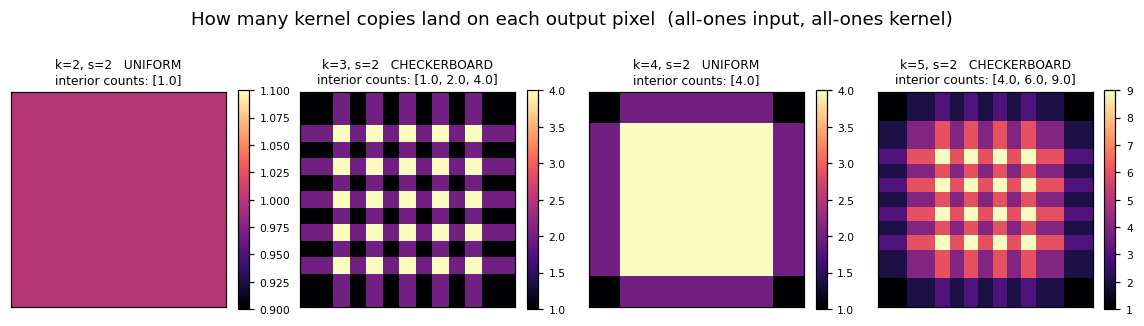
Those overlaps are the catch. Feed an all-ones input through an all-ones kernel: the output value at each position is then literally the number of kernel copies that landed there. If that count is not uniform, the layer multiplies its own output by a fixed periodic pattern, and you get checkerboard artifacts (Odena et al, “Deconvolution and Checkerboard Artifacts”, 2016).

• \(k=3, s=2\): along each axis the counts alternate \(1, 2, 1, 2, \dots\), so in 2D you get \(1, 2, 2, 4\). Bad.

• \(k=4, s=2\): every axis position gets exactly 2 copies, so in 2D every position gets 4. Uniform.

• The rule: stride must divide kernel size. That is why U-Net uses \(k=2, s=2\) and FCN uses \(k=4, s=2\).

def overlap_counts(k, s, n=6):
    """All-ones input through an all-ones kernel: the output IS the count of overlapping copies."""
    x = torch.ones(1, 1, n, n)
    w = torch.ones(1, 1, k, k)
    return F.conv_transpose2d(x, w, stride=s)[0, 0].numpy()

fig, axes = plt.subplots(1, 4, figsize=(10.5, 2.9))
for ax, k in zip(axes, [2, 3, 4, 5]):
    cm = overlap_counts(k, 2)
    interior = cm[k:-k, k:-k]                        # ignore the borders, where counts always taper
    im = ax.imshow(cm, cmap='magma')
    ax.set_title(f'k={k}, s=2   {"UNIFORM" if k % 2 == 0 else "CHECKERBOARD"}\n'
                 f'interior counts: {sorted(set(interior.ravel().tolist()))}', fontsize=8)
    ax.set_xticks([]); ax.set_yticks([])
    plt.colorbar(im, ax=ax, fraction=0.046)
plt.suptitle('How many kernel copies land on each output pixel  (all-ones input, all-ones kernel)', y=1.04)
plt.tight_layout(); plt.show()

print(f'{"kernel":>7} {"stride":>7} {"k % s":>6} {"interior counts":>22} {"uniform?":>9}')
for k in range(2, 7):
    for s in [2, 3]:
        cm = overlap_counts(k, s, n=8)
        interior = cm[2 * k:-2 * k, 2 * k:-2 * k]
        vals = sorted(set(interior.ravel().tolist()))
        print(f'{k:>7} {s:>7} {k % s:>6} {str(vals):>22} {"yes" if len(vals) == 1 else "NO":>9}')
print('\nRule: the overlap is uniform exactly when the stride divides the kernel size (k % s == 0).')

 kernel  stride  k % s        interior counts  uniform?
      2       2      0                  [1.0]       yes
      2       3      2             [0.0, 1.0]        NO
      3       2      1        [1.0, 2.0, 4.0]        NO
      3       3      0                  [1.0]       yes
      4       2      0                  [4.0]       yes
      4       3      1        [1.0, 2.0, 4.0]        NO
      5       2      1                     []        NO
      5       3      2        [1.0, 2.0, 4.0]        NO
      6       2      0                     []        NO
      6       3      0                  [4.0]       yes

Rule: the overlap is uniform exactly when the stride divides the kernel size (k % s == 0).

Interactive: the transpose convolution output size

Move the sliders and watch two things at once:

• the arithmetic \(o = s(i-1) + k - 2p\)

• the overlap-count map, which tells you immediately whether this configuration will checkerboard

def tconv_explorer(input_size=2, kernel=3, stride=2, padding=0):
    o = stride * (input_size - 1) + kernel - 2 * padding
    print(f'o = s(i-1) + k - 2p = {stride}({input_size}-1) + {kernel} - 2({padding}) = {o}')
    if o < 1:
        print(f'   -> output size {o} is not valid: padding crops more than the layer produces. Reduce p.')
        return
    print(f'   {input_size} x {input_size}  ->  {o} x {o}   (scale factor {o/input_size:.2f}x)')
    print(f'   k % s = {kernel % stride}  ->  {"uniform overlap" if kernel % stride == 0 else "UNEVEN overlap: expect checkerboard"}')
    x = torch.ones(1, 1, input_size, input_size)
    w = torch.ones(1, 1, kernel, kernel)
    y = F.conv_transpose2d(x, w, stride=stride, padding=padding)[0, 0].numpy()
    fig, axes = plt.subplots(1, 2, figsize=(6.4, 2.9))
    axes[0].imshow(np.ones((input_size, input_size)), cmap='Blues', vmin=0, vmax=1.6)
    axes[0].set_title(f'input {input_size} x {input_size}')
    im = axes[1].imshow(y, cmap='magma')
    axes[1].set_title(f'output {o} x {o}: overlap counts')
    plt.colorbar(im, ax=axes[1], fraction=0.046)
    for ax in axes:
        ax.set_xticks([]); ax.set_yticks([])
    plt.tight_layout(); plt.show()

widgets.interact(tconv_explorer,
                 input_size=widgets.IntSlider(min=2, max=8, step=1, value=2, continuous_update=False),
                 kernel=widgets.IntSlider(min=1, max=6, step=1, value=3, continuous_update=False),
                 stride=widgets.IntSlider(min=1, max=4, step=1, value=2, continuous_update=False),
                 padding=widgets.IntSlider(min=0, max=3, step=1, value=0, continuous_update=False));

5. FCN with a VGG-16 backbone

Straight from the slide:

• Remove the fully connected layers, replace them with conv layers.

• The last layer has \(C+1\) filters, giving class scores. The spatial size is downsampled by the max-pools.

• One final upsampling layer to get back to the original size (this is FCN-32s).

• Instead of one final upsampling layer, use skip connections from earlier layers for better boundaries.

VGG-16 gives us three useful taps:

tap	stride	\(224 \times 224\) input becomes	character
pool3	8	\(28 \times 28\)	fine, shallow, poor semantics
pool4	16	\(14 \times 14\)	middling
pool5 + conv6/7	32	\(7 \times 7\)	coarse, deep, strong semantics

FCN fuses them by adding score maps (each tap gets its own \(1\times1\) conv to \(C+1\) channels first):

• FCN-32s: upsample the stride-32 score by 32. Coarse.

• FCN-16s: upsample the stride-32 score by 2, add the pool4 score, then upsample by 16.

• FCN-8s: upsample that by 2 again, add the pool3 score, then upsample by 8. Finest.

Note the fusion is a sum, not a concatenation. U-Net will make the other choice, and we will see why it matters.

def vgg_block(cin, cout, n):
    layers = []
    for i in range(n):
        layers += [nn.Conv2d(cin if i == 0 else cout, cout, 3, padding=1), nn.ReLU(inplace=True)]
    return nn.Sequential(*layers)

class TinyVGG16(nn.Module):
    """The VGG-16 layer LAYOUT (2,2,3,3,3 convs and 5 pools) with channel counts divided by 8,
    so it runs instantly on CPU. The strides, which are what this section is about, are identical."""
    def __init__(self, w=8):
        super().__init__()
        self.b1, self.b2 = vgg_block(3, w, 2), vgg_block(w, 2 * w, 2)
        self.b3, self.b4, self.b5 = vgg_block(2 * w, 4 * w, 3), vgg_block(4 * w, 8 * w, 3), vgg_block(8 * w, 8 * w, 3)
    def forward(self, x):
        p1 = F.max_pool2d(self.b1(x), 2)
        p2 = F.max_pool2d(self.b2(p1), 2)
        p3 = F.max_pool2d(self.b3(p2), 2)      # stride 8
        p4 = F.max_pool2d(self.b4(p3), 2)      # stride 16
        p5 = F.max_pool2d(self.b5(p4), 2)      # stride 32
        return p3, p4, p5

class FCN(nn.Module):
    """FCN-32s / 16s / 8s on one backbone. `mode` picks how many skips are fused in."""
    def __init__(self, ncls=NUM_CLASSES, w=8, mode='8s'):
        super().__init__()
        self.mode = mode
        self.backbone = TinyVGG16(w)
        # VGG-16's fc6/fc7/fc8, as convolutions (section 3a). fc6 is 7x7 because pool5 is 7x7.
        self.fc6 = nn.Conv2d(8 * w, 64, 7, padding=3)
        self.fc7 = nn.Conv2d(64, 64, 1)
        self.score5 = nn.Conv2d(64, ncls, 1)               # the "1x1 conv with C+1 channels"
        self.score4 = nn.Conv2d(8 * w, ncls, 1)
        self.score3 = nn.Conv2d(4 * w, ncls, 1)
        self.up2a = nn.ConvTranspose2d(ncls, ncls, 4, stride=2, padding=1)   # k=4,s=2 -> uniform overlap
        self.up2b = nn.ConvTranspose2d(ncls, ncls, 4, stride=2, padding=1)
        self.up32 = nn.ConvTranspose2d(ncls, ncls, 64, stride=32, padding=16)
        self.up16 = nn.ConvTranspose2d(ncls, ncls, 32, stride=16, padding=8)
        self.up8 = nn.ConvTranspose2d(ncls, ncls, 16, stride=8, padding=4)
    def forward(self, x, verbose=False):
        p3, p4, p5 = self.backbone(x)
        s5 = self.score5(F.relu(self.fc7(F.relu(self.fc6(p5)))))
        log = [('input', x), ('pool3 (stride 8)', p3), ('pool4 (stride 16)', p4), ('pool5 (stride 32)', p5),
               ('score from fc7 (stride 32)', s5)]
        if self.mode == '32s':
            out = self.up32(s5)
        else:
            f16 = self.up2a(s5) + self.score4(p4)                       # FUSION IS A SUM
            log += [('upsample x2 + score(pool4) (stride 16)', f16)]
            if self.mode == '16s':
                out = self.up16(f16)
            else:
                f8 = self.up2b(f16) + self.score3(p3)
                log += [('upsample x2 + score(pool3) (stride 8)', f8)]
                out = self.up8(f8)
        log.append((f'final upsample -> FCN-{self.mode}', out))
        if verbose:
            for n, t in log:
                print(f'  {n:44s} {str(tuple(t.shape)):>20s}')
        return out

set_seed()
dummy = torch.randn(1, 3, 224, 224)
for mode in ['32s', '16s', '8s']:
    net = FCN(mode=mode)
    print(f'FCN-{mode}   ({sum(p.numel() for p in net.parameters()):,} params)')
    y = net(dummy, verbose=True)
    assert y.shape[-2:] == dummy.shape[-2:], 'output must be back at input resolution'
    print()
print('All three return the input resolution. They differ only in how much fine detail they can express.')

FCN-32s   (484,672 params)
  input                                            (1, 3, 224, 224)
  pool3 (stride 8)                                  (1, 32, 28, 28)
  pool4 (stride 16)                                 (1, 64, 14, 14)
  pool5 (stride 32)                                   (1, 64, 7, 7)
  score from fc7 (stride 32)                           (1, 3, 7, 7)
  final upsample -> FCN-32s                        (1, 3, 224, 224)

FCN-16s   (484,672 params)
  input                                            (1, 3, 224, 224)
  pool3 (stride 8)                                  (1, 32, 28, 28)
  pool4 (stride 16)                                 (1, 64, 14, 14)
  pool5 (stride 32)                                   (1, 64, 7, 7)
  score from fc7 (stride 32)                           (1, 3, 7, 7)
  upsample x2 + score(pool4) (stride 16)             (1, 3, 14, 14)
  final upsample -> FCN-16s                        (1, 3, 224, 224)

FCN-8s   (484,672 params)
  input                                            (1, 3, 224, 224)
  pool3 (stride 8)                                  (1, 32, 28, 28)
  pool4 (stride 16)                                 (1, 64, 14, 14)
  pool5 (stride 32)                                   (1, 64, 7, 7)
  score from fc7 (stride 32)                           (1, 3, 7, 7)
  upsample x2 + score(pool4) (stride 16)             (1, 3, 14, 14)
  upsample x2 + score(pool3) (stride 8)              (1, 3, 28, 28)
  final upsample -> FCN-8s                         (1, 3, 224, 224)

All three return the input resolution. They differ only in how much fine detail they can express.

What each stride can possibly represent

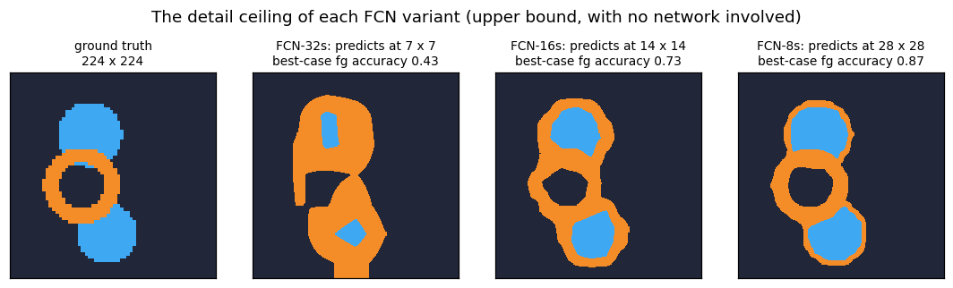
Before training anything, we can measure the detail ceiling of each variant. Take the ground truth mask, squeeze it down to the resolution that variant predicts at (\(7\times7\), \(14\times14\), \(28\times28\) for a \(224\times224\) input), and blow it back up. Even with perfect predictions, this is the best that variant could do.

This is the entire argument for the skip connections, and it needs no training to make.

gt = F.interpolate(Sva[0][None, None].float(), size=(224, 224), mode='nearest')       # a clean 224x224 mask
variants = [('FCN-32s: predicts at 7 x 7', 7), ('FCN-16s: predicts at 14 x 14', 14), ('FCN-8s: predicts at 28 x 28', 28)]

fig, axes = plt.subplots(1, 4, figsize=(10, 2.8))
axes[0].imshow(semantic_rgb(gt[0, 0].long().numpy())); axes[0].set_title('ground truth\n224 x 224')
gt_np = gt[0, 0].long().numpy()
for ax, (name, r) in zip(axes[1:], variants):
    coarse = F.interpolate(gt, size=(r, r), mode='area')                 # what fits in that score map
    back = F.interpolate(coarse, size=(224, 224), mode='bilinear', align_corners=False)
    lab = back[0, 0].round().clamp(0, NUM_CLASSES - 1).long().numpy()
    acc = ((lab == gt_np) & (gt_np > 0)).sum() / max((gt_np > 0).sum(), 1)
    ax.imshow(semantic_rgb(lab)); ax.set_title(f'{name}\nbest-case fg accuracy {acc:.2f}')
for ax in axes:
    ax.set_xticks([]); ax.set_yticks([])
plt.suptitle('The detail ceiling of each FCN variant (upper bound, with no network involved)', y=1.03)
plt.tight_layout(); plt.show()
print('Deeper layers know WHAT the object is. Shallower layers know WHERE its boundary is.')
print('FCN fuses them by summing score maps. SegNet and U-Net will attack the same problem differently.')

Deeper layers know WHAT the object is. Shallower layers know WHERE its boundary is.
FCN fuses them by summing score maps. SegNet and U-Net will attack the same problem differently.

6. SegNet: unpooling with max-pool indices

Badrinarayanan et al, TPAMI 2017. A fully convolutional encoder-decoder:

• the encoder is VGG-16 without the FC layers

• the decoder maps the low-resolution encoder features back to input resolution

• the key idea: the decoder upsamples using the pooling indices stored during the corresponding encoder max-pool

The reasoning:

• A max-pool over a \(2\times2\) window keeps one value and remembers which of the 4 positions it came from (the index).

• On the way up, SegNet places each value back at its original position and fills the other 3 with zeros. This is unpooling, and it produces a sparse map.

• Conv layers after the unpooling densify the sparse map.

• Storing indices is cheap. You keep 2 bits per pooled element (which of 4), not a whole float feature map, so the decoder recovers boundary locations almost for free.

PyTorch gives us exactly the two pieces: F.max_pool2d(..., return_indices=True) and nn.MaxUnpool2d.

6a. Reproducing the exact figure from the slide

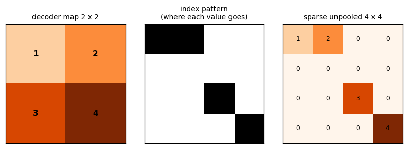
The slide shows a \(2\times2\) decoder map \(\begin{smallmatrix}a&b\\c&d\end{smallmatrix}\) and an index map, and puts each of \(a, b, c, d\) into the remembered corner of its \(2\times2\) output window. Let us reproduce it value for value.

# the decoder map from the slide
dec = torch.tensor([[[[1., 2.], [3., 4.]]]])                     # a=1, b=2, c=3, d=4

# the slide's index pattern: a->top-left(0), b->top-right(1), c->bottom-left(2), d->bottom-right(3)
# (flattened-window index, which is what nn.MaxUnpool2d consumes)
idx = torch.tensor([[[[0, 1], [10, 15]]]])

unpool = nn.MaxUnpool2d(kernel_size=2, stride=2)
sparse = unpool(dec, idx, output_size=(4, 4))[0, 0]
print('decoder map (from prev decoder stage):')
print(dec[0, 0].int().numpy())
print('\nunpooled to 4 x 4 using the stored max-pool indices (0s elsewhere):')
print(sparse.int().numpy())
print('\nEach value landed in its remembered corner. This matches the slide exactly.')
print('A conv layer would now run over this sparse map to fill the zeros (densify).')

fig, axes = plt.subplots(1, 3, figsize=(7.5, 2.6))
axes[0].imshow(dec[0, 0], cmap='Oranges', vmin=0, vmax=4)
axes[0].set_title('decoder map 2 x 2')
for i in range(2):
    for j in range(2):
        axes[0].text(j, i, f'{int(dec[0,0,i,j])}', ha='center', va='center', fontweight='bold')
axes[1].imshow((sparse > 0).float(), cmap='Greys', vmin=0, vmax=1)
axes[1].set_title('index pattern\n(where each value goes)')
axes[2].imshow(sparse, cmap='Oranges', vmin=0, vmax=4)
axes[2].set_title('sparse unpooled 4 x 4')
for i in range(4):
    for j in range(4):
        axes[2].text(j, i, f'{int(sparse[i,j])}', ha='center', va='center', fontsize=8)
for ax in axes:
    ax.set_xticks([]); ax.set_yticks([])
plt.tight_layout(); plt.show()

decoder map (from prev decoder stage):
[[1 2]
 [3 4]]

unpooled to 4 x 4 using the stored max-pool indices (0s elsewhere):
[[1 2 0 0]
 [0 0 0 0]
 [0 0 3 0]
 [0 0 0 4]]

Each value landed in its remembered corner. This matches the slide exactly.
A conv layer would now run over this sparse map to fill the zeros (densify).

6b. Why indices beat blind upsampling: a real max-unpool round trip

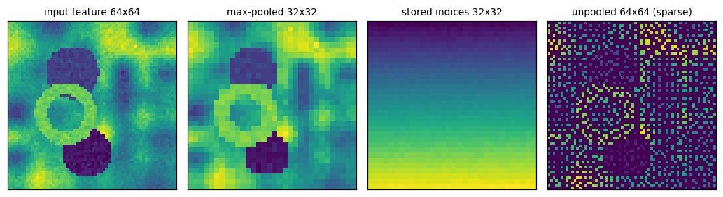
We pool a real feature (the image’s green channel), throw away everything except the kept values and their indices, and then unpool. Because the indices remember where the maxima were, the reconstruction lands energy back on the true high-response locations (edges), which a fixed upsampler cannot know.

feat = Xva[0, 1][None, None]                                     # green channel, (1,1,64,64)
pooled, indices = F.max_pool2d(feat, 2, stride=2, return_indices=True)
unpooled = F.max_unpool2d(pooled, indices, 2, stride=2)
print(f'feature {tuple(feat.shape[2:])} -> pooled {tuple(pooled.shape[2:])} (+ int index map) -> unpooled {tuple(unpooled.shape[2:])}')
print(f'the index map stores 1 integer per pooled cell: {indices.numel()} ints, vs {feat.numel()} floats for the full map')

fig, axes = plt.subplots(1, 4, figsize=(9.5, 2.6))
for ax, im, t in zip(axes, [feat, pooled, indices.float(), unpooled],
                     ['input feature 64x64', 'max-pooled 32x32', 'stored indices 32x32', 'unpooled 64x64 (sparse)']):
    m = ax.imshow(im[0, 0], cmap='viridis'); ax.set_title(t); ax.set_xticks([]); ax.set_yticks([])
plt.tight_layout(); plt.show()
print('The unpooled map is sparse (3/4 of cells are 0) but its non-zeros sit exactly on the original maxima.')

feature (64, 64) -> pooled (32, 32) (+ int index map) -> unpooled (64, 64)
the index map stores 1 integer per pooled cell: 1024 ints, vs 4096 floats for the full map
The unpooled map is sparse (3/4 of cells are 0) but its non-zeros sit exactly on the original maxima.

6c. Three ways to upsample, side by side

We now have three upsampling strategies on the table. Applied to the same low-resolution feature:

Method	Learnable?	What it does
Nearest / bilinear interpolation	no	fixed averaging rule, blurs boundaries (used inside PSPNet, DeepLab)
Transpose convolution	yes	learns a scatter kernel (used in FCN, U-Net)
Max-unpool with indices	no (but uses encoder info)	places values back where the maxima were (used in SegNet)

The interactive selector lets you switch between them on our feature map.

small = F.avg_pool2d(Xva[0, 1][None, None], 8)                   # 8x8 low-res feature to upsample back to 64

def upsample_demo(method='bilinear'):
    if method == 'nearest':
        up = F.interpolate(small, size=(64, 64), mode='nearest')
    elif method == 'bilinear':
        up = F.interpolate(small, size=(64, 64), mode='bilinear', align_corners=False)
    elif method == 'transpose conv (random init)':
        set_seed(); layer = nn.ConvTranspose2d(1, 1, 8, stride=8); up = layer(small).detach()
    elif method == 'max-unpool (indices)':
        big = Xva[0, 1][None, None]
        _, idx = F.max_pool2d(big, 8, stride=8, return_indices=True)
        up = F.max_unpool2d(small, idx, 8, stride=8)
    fig, axes = plt.subplots(1, 3, figsize=(7.2, 2.6))
    axes[0].imshow(small[0, 0], cmap='viridis'); axes[0].set_title('8 x 8 feature')
    axes[1].imshow(up[0, 0], cmap='viridis'); axes[1].set_title(f'{method}\n-> 64 x 64')
    axes[2].imshow(Xva[0, 1], cmap='viridis'); axes[2].set_title('original 64 x 64')
    for ax in axes:
        ax.set_xticks([]); ax.set_yticks([])
    plt.tight_layout(); plt.show()

widgets.interact(upsample_demo,
                 method=widgets.Dropdown(options=['nearest', 'bilinear', 'transpose conv (random init)',
                                                  'max-unpool (indices)'], value='bilinear'));

7. U-Net, built block by block

Ronneberger et al, MICCAI 2015. The slide describes it as a fully convolutional encoder-decoder with skip connections, an extension of FCN. The differences from FCN that matter:

• the skip is a concatenation, not a sum (FCN summed score maps; U-Net concatenates features)

• the expanding path has many feature channels, so it can carry rich information upward

• concatenating encoder features gives the decoder localization information: what comes up from the bottleneck, where comes across from the encoder

• the slide notes summing is an alternative to concatenation (that alternative is essentially FCN’s fusion)

U-Net specifics from the slides, which we honour where it is cheap to:

• upsampling by a \(2\times2\) transpose conv, stride 2, padding 0, halving channels and doubling spatial size

• final layer is a \(1\times1\) conv with \(C+1\) channels

• the original uses unpadded convs, so the output is smaller than the input by a border; we use padded convs so shapes stay tidy for teaching (a common modern choice)

We build three Lego bricks: DoubleConv, a down step, an up step. Then we stack them.

class DoubleConv(nn.Module):
    """(conv 3x3 -> BN -> ReLU) x 2. The repeating unit of both paths."""
    def __init__(self, cin, cout):
        super().__init__()
        self.net = nn.Sequential(
            nn.Conv2d(cin, cout, 3, padding=1, bias=False), nn.BatchNorm2d(cout), nn.ReLU(inplace=True),
            nn.Conv2d(cout, cout, 3, padding=1, bias=False), nn.BatchNorm2d(cout), nn.ReLU(inplace=True))
    def forward(self, x):
        return self.net(x)

class Down(nn.Module):
    """Contracting step: max-pool by 2, then DoubleConv. Halves H,W and (usually) doubles channels."""
    def __init__(self, cin, cout):
        super().__init__()
        self.pool = nn.MaxPool2d(2)
        self.conv = DoubleConv(cin, cout)
    def forward(self, x):
        return self.conv(self.pool(x))

class Up(nn.Module):
    """Expanding step: 2x2 transpose conv (up), CONCATENATE the encoder skip, then DoubleConv."""
    def __init__(self, cin, cout, use_skip=True):
        super().__init__()
        self.use_skip = use_skip
        self.up = nn.ConvTranspose2d(cin, cout, kernel_size=2, stride=2)     # k=2,s=2: no checkerboard
        self.conv = DoubleConv(cout * 2, cout)                              # *2 because of the concat
    def forward(self, x, skip):
        x = self.up(x)
        if not self.use_skip:
            skip = torch.zeros_like(skip)                                   # ablation: keep shapes, drop information
        return self.conv(torch.cat([x, skip], dim=1))

# sanity-check one Up block's shapes, including the concatenation
set_seed()
up = Up(16, 8)
x_lo = torch.randn(1, 16, 8, 8)
skip = torch.randn(1, 8, 16, 16)
print(f'bottleneck feature {tuple(x_lo.shape)}')
print(f'  transpose-conv up 2x   -> {tuple(up.up(x_lo).shape)}')
print(f'  encoder skip           {tuple(skip.shape)}')
print(f'  concat -> DoubleConv   -> {tuple(up(x_lo, skip).shape)}   (channels: 8 up + 8 skip = 16 in, 8 out)')

bottleneck feature (1, 16, 8, 8)
  transpose-conv up 2x   -> (1, 8, 16, 16)
  encoder skip           (1, 8, 16, 16)
  concat -> DoubleConv   -> (1, 8, 16, 16)   (channels: 8 up + 8 skip = 16 in, 8 out)

7a. Assembling the U, and printing every shape

The generic U-Net below takes a base channel width and a depth, and a use_skips flag we will need for the ablation. We forward one image with verbose=True so you can read the spatial size contract then expand, and see each skip tensor being carried across at matching resolution.

class UNet(nn.Module):
    def __init__(self, cin=3, ncls=NUM_CLASSES, base=8, depth=3, use_skips=True):
        super().__init__()
        self.depth, self.use_skips = depth, use_skips
        chs = [base * (2 ** i) for i in range(depth + 1)]       # e.g. base=8, depth=3 -> [8,16,32,64]
        self.inc = DoubleConv(cin, chs[0])
        self.downs = nn.ModuleList([Down(chs[i], chs[i + 1]) for i in range(depth)])
        self.ups = nn.ModuleList([Up(chs[i + 1], chs[i], use_skips) for i in reversed(range(depth))])
        self.outc = nn.Conv2d(chs[0], ncls, 1)                  # final 1x1 conv, C+1 channels
    def forward(self, x, verbose=False):
        skips = [self.inc(x)]
        if verbose:
            print(f'  {"inc":16s} {str(tuple(skips[-1].shape)):>22s}')
        for i, d in enumerate(self.downs):
            skips.append(d(skips[-1]))
            if verbose:
                print(f'  {"down " + str(i + 1):16s} {str(tuple(skips[-1].shape)):>22s}  (contracting)')
        x = skips[-1]
        for i, up in enumerate(self.ups):
            skip = skips[self.depth - 1 - i]
            x = up(x, skip)
            if verbose:
                tag = 'concat skip ' + str(tuple(skip.shape)[1:]) if self.use_skips else 'skip DROPPED'
                print(f'  {"up " + str(i + 1):16s} {str(tuple(x.shape)):>22s}  (expanding, {tag})')
        out = self.outc(x)
        if verbose:
            print(f'  {"outc (1x1)":16s} {str(tuple(out.shape)):>22s}  <- {NUM_CLASSES} class scores per pixel')
        return out

set_seed()
unet = UNet(base=8, depth=3).to(device)
print(f'Tiny U-Net: base=8, depth=3, {sum(p.numel() for p in unet.parameters()):,} parameters\n')
print('forward pass shapes (input 3 x 64 x 64):')
_ = unet(Xva[:1].to(device), verbose=True)

Tiny U-Net: base=8, depth=3, 121,195 parameters

forward pass shapes (input 3 x 64 x 64):
  inc                      (1, 8, 64, 64)
  down 1                  (1, 16, 32, 32)  (contracting)
  down 2                  (1, 32, 16, 16)  (contracting)
  down 3                    (1, 64, 8, 8)  (contracting)
  up 1                    (1, 32, 16, 16)  (expanding, concat skip (32, 16, 16))
  up 2                    (1, 16, 32, 32)  (expanding, concat skip (16, 32, 32))
  up 3                     (1, 8, 64, 64)  (expanding, concat skip (8, 64, 64))
  outc (1x1)               (1, 3, 64, 64)  <- 3 class scores per pixel

7b. A picture of the U

The shape table above is the U-Net “U” written out in numbers. Here it is as a diagram: the contracting path on the left, the expanding path on the right, the bottleneck at the bottom, and the grey concatenation skips crossing at each level. This is the figure from the slides, drawn from our own channel and resolution numbers.

def _box(ax, x, y, h, fc, ec):
    ax.add_patch(mpatches.FancyBboxPatch((x, y - h / 2), 0.5, h,
                 boxstyle='round,pad=0.02', fc=fc, ec=ec, mutation_aspect=0.6))

def draw_unet(base=8, depth=3, H=64):
    chs = [base * (2 ** i) for i in range(depth + 1)]
    res = [H // (2 ** i) for i in range(depth + 1)]
    fig, ax = plt.subplots(figsize=(9.5, 5.2))
    encx = [0.6 + 0.15 * lvl for lvl in range(depth + 1)]
    decx = [3.4 - 0.15 * lvl for lvl in range(depth + 1)]
    for lvl in range(depth + 1):                                       # encoder column (left)
        y, h = -lvl, 0.30 + 0.5 * res[lvl] / H
        _box(ax, encx[lvl], y, h, '#8ecae6', '#023047')
        ax.text(encx[lvl] + 0.25, y, f'{res[lvl]}x{res[lvl]}\n{chs[lvl]}c', ha='center', va='center', fontsize=7)
        if lvl < depth:
            ax.text(encx[lvl] + 0.25, y - 0.5, 'pool', ha='center', va='center', fontsize=6.5, color='0.3')
    for lvl in range(depth):                                           # decoder column (right)
        y, h = -lvl, 0.30 + 0.5 * res[lvl] / H
        _box(ax, decx[lvl], y, h, '#ffb703', '#fb8500')
        ax.text(decx[lvl] + 0.25, y, f'{res[lvl]}x{res[lvl]}\n{chs[lvl]}c', ha='center', va='center', fontsize=7)
        ax.annotate('', xy=(decx[lvl], y), xytext=(encx[lvl] + 0.5, y),   # concatenation skip
                    arrowprops=dict(arrowstyle='-|>', color='0.45', lw=1.4, ls='--'))
        ax.text((encx[lvl] + 0.5 + decx[lvl]) / 2, y + 0.12, 'concat', ha='center', fontsize=6.5, color='0.4')
    for lvl in range(depth):                                           # decoder up arrows
        ax.annotate('', xy=(decx[lvl] + 0.25, -lvl - 0.35),
                    xytext=(decx[min(lvl + 1, depth - 1)] + 0.25, -lvl - 0.65),
                    arrowprops=dict(arrowstyle='-|>', color='#fb8500', lw=1.2))
    ax.text(encx[0] + 0.25, 0.75, 'input\nimage', ha='center', fontsize=8)
    ax.text(decx[0] + 0.25, 0.75, 'C+1 scores\nper pixel', ha='center', fontsize=8)
    ax.text(2.0, -depth + 0.15, 'bottleneck', ha='center', fontsize=8, color='0.3')
    ax.text(1.1, 0.55, 'contracting (encoder)', fontsize=8, color='#023047')
    ax.text(2.7, 0.55, 'expanding (decoder)', fontsize=8, color='#fb8500')
    ax.set_xlim(0.2, 4.2); ax.set_ylim(-depth - 0.9, 1.1); ax.axis('off')
    ax.set_title(f'U-Net: base={base}, depth={depth}  (grey dashed = concatenation skips)')
    plt.tight_layout(); plt.show()

draw_unet(base=8, depth=3)

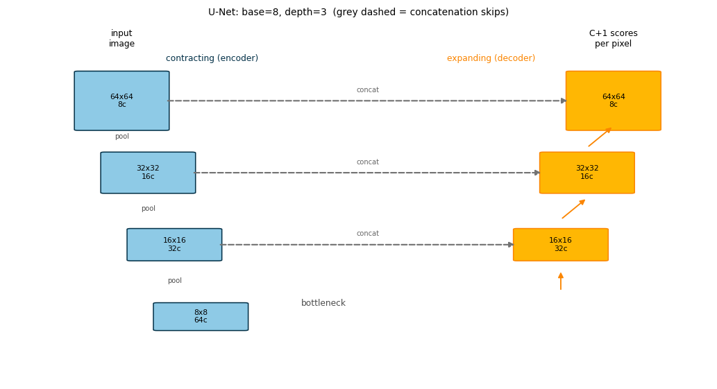
Interactive: architecture introspection (no training)

Move the sliders to see how base (channel width) and depth change the parameter count and the shape table. This is pure architecture bookkeeping, instantaneous, no training. It builds intuition for the classic trade-off: depth buys a larger receptive field and more abstraction, width buys capacity, both cost parameters (and memory) quadratically in base.

def unet_introspect(base=8, depth=3):
    net = UNet(base=base, depth=depth)
    n = sum(p.numel() for p in net.parameters())
    chs = [base * (2 ** i) for i in range(depth + 1)]
    res = [64 // (2 ** i) for i in range(depth + 1)]
    print(f'base={base}  depth={depth}  ->  {n:,} parameters   (bottleneck: {res[-1]} x {res[-1]}, {chs[-1]} channels)')
    print(f'\n{"level":>6} {"encoder res":>13} {"channels":>10}')
    for i in range(depth + 1):
        print(f'{i:>6} {str(res[i]) + " x " + str(res[i]):>13} {chs[i]:>10}')
    with torch.no_grad():
        _ = net(torch.zeros(1, 3, 64, 64))          # confirm it runs at this configuration
    print('\nforward pass OK at this configuration.')

widgets.interact(unet_introspect,
                 base=widgets.IntSlider(min=4, max=24, step=4, value=8, continuous_update=False),
                 depth=widgets.IntSlider(min=1, max=4, step=1, value=3, continuous_update=False));

7c. A metric to watch: mean IoU

Pixel accuracy is a poor segmentation metric because the background dominates: a network that predicts “all background” already scores over 75% here. Intersection over Union does not have that loophole. We build the full multi-class version now (from a confusion matrix) and reuse it as our training metric; section 17 re-derives IoU and its cousins from scratch.

def confusion_matrix(pred, gt, n):
    """Fast confusion matrix via bincount. pred, gt: integer label tensors of any matching shape."""
    k = (gt.reshape(-1) * n + pred.reshape(-1))
    return torch.bincount(k, minlength=n * n).reshape(n, n).float()

def iou_per_class(cm):
    inter = cm.diag()
    union = cm.sum(0) + cm.sum(1) - inter
    return inter / union.clamp(min=1e-6), union

def mean_iou(cm):
    ious, union = iou_per_class(cm)
    valid = union > 0
    return ious[valid].mean().item()

@torch.no_grad()
def evaluate(model, X, Y, bs=32):
    model.eval()
    cm = torch.zeros(NUM_CLASSES, NUM_CLASSES)
    for i in range(0, len(X), bs):
        pred = model(X[i:i + bs].to(device)).argmax(1).cpu()
        cm += confusion_matrix(pred, Y[i:i + bs], NUM_CLASSES)
    model.train()
    return mean_iou(cm), cm

# a "predict all background" baseline, to show why we do not use pixel accuracy
allbg = torch.zeros_like(Sva)
print(f'trivial "all background" predictor:')
print(f'  pixel accuracy = {(allbg == Sva).float().mean():.3f}   (looks great, means nothing)')
print(f'  mean IoU       = {mean_iou(confusion_matrix(allbg, Sva, NUM_CLASSES)):.3f}   (correctly near {1/3:.2f}: it gets 1 of 3 classes)')

trivial "all background" predictor:
  pixel accuracy = 0.783   (looks great, means nothing)
  mean IoU       = 0.261   (correctly near 0.33: it gets 1 of 3 classes)

7d. Train the tiny U-Net

The recipe, chosen so it converges reliably on a CPU in well under a minute:

• 256 synthetic training images, batch size 8, 450 steps (about 14 epochs)

• Adam, learning rate \(3\times10^{-3}\), cosine decay with a short warm-up

• plain pixel-wise cross-entropy, exactly as the slides specify

We snapshot the validation mIoU and the predicted masks at several steps so we can watch learning happen.

SNAP_STEPS = [0, 50, 150, 300, 450]

def make_scheduler(opt, steps, warm=50):
    def f(s):
        if s < warm:
            return (s + 1) / warm
        return 0.5 * (1 + math.cos(math.pi * (s - warm) / max(1, steps - warm)))
    return torch.optim.lr_scheduler.LambdaLR(opt, f)

def train_unet(model, steps=450, bs=8, lr=3e-3, log_every=50, snap=None, verbose=True):
    model.to(device).train()
    opt = torch.optim.Adam(model.parameters(), lr=lr)
    sched = make_scheduler(opt, steps)
    gen = torch.Generator().manual_seed(SEED)
    curve, snaps = [], {}
    t0 = time.time()
    for s in range(steps + 1):
        if s % log_every == 0 or s == steps:
            miou, _ = evaluate(model, Xva, Sva)
            curve.append((s, miou))
            if snap is not None and s in snap:
                with torch.no_grad():
                    snaps[s] = model(Xva[:4].to(device)).argmax(1).cpu().numpy()
            if verbose:
                print(f'  step {s:4d}   val mIoU {miou:.3f}   ({time.time()-t0:4.1f}s)')
        if s == steps:
            break
        idx = torch.randint(0, len(Xtr), (bs,), generator=gen)
        logits = model(Xtr[idx].to(device))
        loss = F.cross_entropy(logits, Str[idx].to(device))
        opt.zero_grad(); loss.backward(); opt.step(); sched.step()
    return curve, snaps, time.time() - t0

print('training U-Net WITH skip connections ...')
set_seed()
unet_skip = UNet(base=8, depth=3, use_skips=True)
curve_skip, snaps_skip, t_skip = train_unet(unet_skip, snap=SNAP_STEPS)
miou_skip = curve_skip[-1][1]
print(f'done in {t_skip:.1f}s   final val mIoU = {miou_skip:.3f}')

training U-Net WITH skip connections ...
  step    0   val mIoU 0.027   ( 0.1s)
  step   50   val mIoU 0.091   ( 0.9s)
  step  100   val mIoU 0.630   ( 1.6s)
  step  150   val mIoU 0.769   ( 2.3s)
  step  200   val mIoU 0.825   ( 3.1s)
  step  250   val mIoU 0.845   ( 3.8s)
  step  300   val mIoU 0.842   ( 4.6s)
  step  350   val mIoU 0.856   ( 5.3s)
  step  400   val mIoU 0.861   ( 6.1s)
  step  450   val mIoU 0.865   ( 6.8s)
done in 6.8s   final val mIoU = 0.865

7e. Watching the masks sharpen

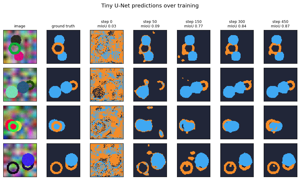
Same network, five checkpoints. The prediction goes from random noise, through recognisable blobs, to crisp shapes with hollow ring centres. The ring holes are the tell: reconstructing them requires fine spatial information, which the concatenation skips deliver from the encoder.

fig, axes = plt.subplots(4, len(SNAP_STEPS) + 2, figsize=(1.35 * (len(SNAP_STEPS) + 2), 5.4))
for r in range(4):
    axes[r, 0].imshow(Xva[r].numpy().transpose(1, 2, 0))
    axes[r, 1].imshow(semantic_rgb(Sva[r].numpy()))
    for c, s in enumerate(SNAP_STEPS):
        axes[r, c + 2].imshow(semantic_rgb(snaps_skip[s][r]))
for c, t in enumerate(['image', 'ground truth'] + [f'step {s}\nmIoU {dict(curve_skip)[s]:.2f}' for s in SNAP_STEPS]):
    axes[0, c].set_title(t, fontsize=8)
for ax in axes.ravel():
    ax.set_xticks([]); ax.set_yticks([])
plt.suptitle('Tiny U-Net predictions over training', y=1.01)
plt.tight_layout(); plt.show()

7f. The skip-connection ablation (a real measured result)

Now the experiment the slides motivate but cannot run. We train the identical network with the skips zeroed out. Everything else is held fixed: same architecture, same parameter count, same seed, same optimiser, same 450 steps. The transpose-conv upsampling is still there, so the decoder can still upsample; it just no longer receives the encoder’s fine-detail features.

This is a toy-scale result (a small net, a small synthetic dataset, a few hundred CPU steps), so read the trend, not the decimals. We report exactly what we measured.

print('training U-Net WITHOUT skip connections (ablation) ...')
set_seed()
unet_noskip = UNet(base=8, depth=3, use_skips=False)
curve_noskip, snaps_noskip, t_noskip = train_unet(unet_noskip, snap=[450])
miou_noskip = curve_noskip[-1][1]

# boundary-band mIoU: restrict the metric to pixels near a semantic edge, where skips should help most
def boundary_band(gt, width=2):
    oh = F.one_hot(gt, NUM_CLASSES).permute(0, 3, 1, 2).float()
    dil = F.max_pool2d(oh, 2 * width + 1, 1, width)
    ero = -F.max_pool2d(-oh, 2 * width + 1, 1, width)
    return (dil - ero).sum(1) > 0

@torch.no_grad()
def band_miou(model):
    model.eval()
    cm = torch.zeros(NUM_CLASSES, NUM_CLASSES)
    for i in range(0, len(Xva), 32):
        g = Sva[i:i + 32]
        p = model(Xva[i:i + 32].to(device)).argmax(1).cpu()
        b = boundary_band(g)
        cm += confusion_matrix(p[b], g[b], NUM_CLASSES)
    model.train()
    return mean_iou(cm)

band_skip, band_noskip = band_miou(unet_skip), band_miou(unet_noskip)
print(f'\n{"":22s} {"overall mIoU":>13} {"boundary mIoU":>14}')
print(f'{"WITH skips":22s} {miou_skip:>13.3f} {band_skip:>14.3f}')
print(f'{"WITHOUT skips":22s} {miou_noskip:>13.3f} {band_noskip:>14.3f}')
print(f'{"difference":22s} {miou_skip-miou_noskip:>+13.3f} {band_skip-band_noskip:>+14.3f}')
print('\nThe gap is real and it is larger at boundaries, which is exactly where fine detail lives.')

training U-Net WITHOUT skip connections (ablation) ...
  step    0   val mIoU 0.027   ( 0.1s)
  step   50   val mIoU 0.214   ( 0.8s)
  step  100   val mIoU 0.529   ( 1.6s)
  step  150   val mIoU 0.550   ( 2.3s)
  step  200   val mIoU 0.552   ( 3.1s)
  step  250   val mIoU 0.565   ( 3.8s)
  step  300   val mIoU 0.569   ( 4.5s)
  step  350   val mIoU 0.595   ( 5.3s)
  step  400   val mIoU 0.637   ( 6.0s)
  step  450   val mIoU 0.658   ( 6.8s)

                        overall mIoU  boundary mIoU
WITH skips                     0.865          0.792
WITHOUT skips                  0.658          0.512
difference                    +0.207         +0.281

The gap is real and it is larger at boundaries, which is exactly where fine detail lives.

The ablation, as pictures

Side by side on the same images. Look at the ring centres and the edges: with skips the holes are open and the boundaries are clean; without skips the decoder, working only from the coarse bottleneck, tends to fill holes and round off the thin ring walls.

fig, axes = plt.subplots(4, 4, figsize=(7.6, 7.4))
for r in range(4):
    axes[r, 0].imshow(Xva[r].numpy().transpose(1, 2, 0))
    axes[r, 1].imshow(semantic_rgb(Sva[r].numpy()))
    axes[r, 2].imshow(semantic_rgb(snaps_skip[450][r]))
    axes[r, 3].imshow(semantic_rgb(snaps_noskip[450][r]))
for c, t in enumerate(['image', 'ground truth', f'WITH skips\nmIoU {miou_skip:.2f}',
                       f'WITHOUT skips\nmIoU {miou_noskip:.2f}']):
    axes[0, c].set_title(t, fontsize=8.5)
for ax in axes.ravel():
    ax.set_xticks([]); ax.set_yticks([])
plt.tight_layout(); plt.show()

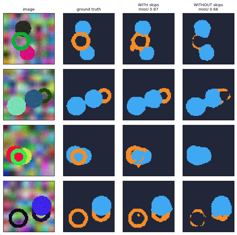
Training curves

Both curves, plus the boundary-mIoU bars. The skip network reaches a higher mIoU and gets there faster, because it does not have to learn to hallucinate detail it threw away at the bottleneck.

fig, axes = plt.subplots(1, 2, figsize=(9.5, 3.2))
axes[0].plot(*zip(*curve_skip), 'o-', label=f'with skips (final {miou_skip:.3f})', color='#0077b6')
axes[0].plot(*zip(*curve_noskip), 's--', label=f'without skips (final {miou_noskip:.3f})', color='#e63946')
axes[0].set_xlabel('training step'); axes[0].set_ylabel('validation mIoU')
axes[0].set_title('U-Net training: skip vs no-skip'); axes[0].legend(); axes[0].grid(alpha=0.3)
bars = axes[1].bar(['overall\nwith', 'overall\nwithout', 'boundary\nwith', 'boundary\nwithout'],
                   [miou_skip, miou_noskip, band_skip, band_noskip],
                   color=['#0077b6', '#e63946', '#0077b6', '#e63946'], alpha=0.85)
axes[1].set_ylabel('mIoU'); axes[1].set_title('overall vs boundary mIoU'); axes[1].grid(alpha=0.3, axis='y')
for b, v in zip(bars, [miou_skip, miou_noskip, band_skip, band_noskip]):
    axes[1].text(b.get_x() + b.get_width() / 2, v + 0.01, f'{v:.2f}', ha='center', fontsize=8)
plt.tight_layout(); plt.show()

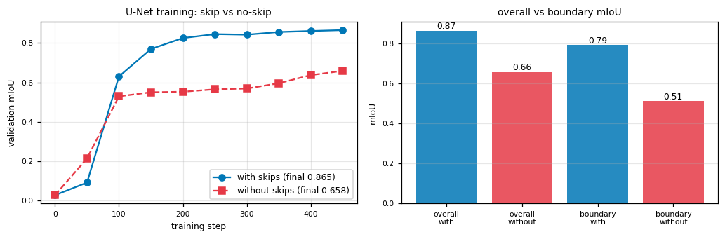
Interactive: the decision threshold on the trained U-Net

The network outputs a probability per class per pixel. Turning those probabilities into a mask needs a rule. Here we sweep a foreground-probability threshold: a pixel is called foreground only if \(P(\text{foreground}) = 1 - P(\text{background})\) exceeds the threshold, and is then assigned the more likely of the two thing classes. Watch the live mIoU and the mask trade blame between false positives (low threshold) and false negatives (high threshold).

with torch.no_grad():
    val_probs = F.softmax(unet_skip(Xva.to(device)), dim=1).cpu()          # (N, C, H, W), computed once

def threshold_explorer(fg_threshold=0.50, image=0):
    probs = val_probs
    fg_prob = 1 - probs[:, 0]                                              # P(not background)
    is_fg = fg_prob > fg_threshold
    thing = probs[:, 1:].argmax(1) + 1                                     # ring vs disk among fg
    pred = torch.where(is_fg, thing, torch.zeros_like(thing))
    miou = mean_iou(confusion_matrix(pred, Sva, NUM_CLASSES))
    fig, axes = plt.subplots(1, 4, figsize=(9.5, 2.6))
    axes[0].imshow(Xva[image].numpy().transpose(1, 2, 0)); axes[0].set_title('image')
    axes[1].imshow(fg_prob[image], cmap='magma', vmin=0, vmax=1); axes[1].set_title('P(foreground)')
    axes[2].imshow(semantic_rgb(pred[image].numpy())); axes[2].set_title(f'pred @ thr {fg_threshold:.2f}')
    axes[3].imshow(semantic_rgb(Sva[image].numpy())); axes[3].set_title('ground truth')
    for ax in axes:
        ax.set_xticks([]); ax.set_yticks([])
    plt.suptitle(f'dataset-wide mIoU at this threshold = {miou:.3f}', y=1.04)
    plt.tight_layout(); plt.show()

widgets.interact(threshold_explorer,
                 fg_threshold=widgets.FloatSlider(min=0.05, max=0.95, step=0.05, value=0.50, continuous_update=False),
                 image=widgets.IntSlider(min=0, max=7, step=1, value=0, continuous_update=False));

8. PSPNet: the pyramid pooling module

Zhao et al, CVPR 2017. The slide first lists what can go wrong when a plain FCN meets a complex scene:

• it may miss that some patterns co-occur: cars on roads, boats on rivers (a boat-shaped thing on a road is probably a car)

• it may label parts of one object as different categories (part of a skyscraper read as a different building)

• it may mishandle objects that are very large or very small relative to its receptive field

The common cause is a lack of global context. PSPNet’s fix, the Pyramid Pooling Module (PPM):

• take the final feature map of a deep backbone (ResNet), with \(c\) channels

• average-pool it at four scales: \(1\times1\) (this is global average pooling, the coarsest), \(2\times2\), \(3\times3\), \(6\times6\)

• a \(1\times1\) conv reduces each pooled level to \(c/4\) channels (4 levels, so the totals stay balanced)

• bilinearly upsample every level back to the feature map’s size

• concatenate the four upsampled maps with the original feature map

• a final conv fuses everything and predicts

Each level answers a different question: the \(1\times1\) level says “what is in this scene overall”, the \(6\times6\) level says “what is in this general region”. Let us build it from scratch and watch the shapes at every scale.

class PyramidPoolingModule(nn.Module):
    def __init__(self, in_ch, scales=(1, 2, 3, 6)):
        super().__init__()
        self.scales = scales
        red = in_ch // len(scales)                              # c/4
        self.branches = nn.ModuleList([
            nn.Sequential(nn.AdaptiveAvgPool2d(s), nn.Conv2d(in_ch, red, 1), nn.ReLU(inplace=True))
            for s in scales])
        self.fuse = nn.Conv2d(in_ch + red * len(scales), in_ch, 3, padding=1)
    def forward(self, x, verbose=False):
        H, W = x.shape[-2:]
        feats = [x]
        if verbose:
            print(f'  backbone feature map           {str(tuple(x.shape)):>22s}')
        for s, br in zip(self.scales, self.branches):
            pooled = br[0](x)                                   # adaptive avg pool to s x s
            reduced = br[2](br[1](pooled))                      # 1x1 conv -> c/4, then ReLU
            up = F.interpolate(reduced, size=(H, W), mode='bilinear', align_corners=False)
            feats.append(up)
            if verbose:
                print(f'  level {s} x {s}: pool {str(tuple(pooled.shape[1:])):>12s} '
                      f'-> 1x1 conv {str(tuple(reduced.shape[1:])):>10s} -> upsample {tuple(up.shape[2:])}')
        cat = torch.cat(feats, dim=1)
        out = self.fuse(cat)
        if verbose:
            print(f'  concatenate [original + 4 levels] {str(tuple(cat.shape)):>19s}')
            print(f'  fuse conv -> output               {str(tuple(out.shape)):>19s}')
        return out

set_seed()
backbone_feat = torch.randn(1, 16, 12, 12)                     # pretend this is ResNet's stride-32 feature map, c=16
ppm = PyramidPoolingModule(16)
print('Pyramid Pooling Module, scales (1, 2, 3, 6):\n')
_ = ppm(backbone_feat, verbose=True)
print('\nEach level pools to a fixed grid regardless of input size, so the module sees the whole scene at 4 granularities.')

Pyramid Pooling Module, scales (1, 2, 3, 6):

  backbone feature map                  (1, 16, 12, 12)
  level 1 x 1: pool   (16, 1, 1) -> 1x1 conv  (4, 1, 1) -> upsample (12, 12)
  level 2 x 2: pool   (16, 2, 2) -> 1x1 conv  (4, 2, 2) -> upsample (12, 12)
  level 3 x 3: pool   (16, 3, 3) -> 1x1 conv  (4, 3, 3) -> upsample (12, 12)
  level 6 x 6: pool   (16, 6, 6) -> 1x1 conv  (4, 6, 6) -> upsample (12, 12)
  concatenate [original + 4 levels]     (1, 32, 12, 12)
  fuse conv -> output                   (1, 16, 12, 12)

Each level pools to a fixed grid regardless of input size, so the module sees the whole scene at 4 granularities.

The four pyramid levels, visualised

The same feature map, average-pooled to \(1\times1\), \(2\times2\), \(3\times3\), \(6\times6\). The \(1\times1\) level is a single global summary; each finer level keeps a little more spatial (“localization”) information, exactly as the slide says.

feat_vis = F.avg_pool2d(Xva[0, 1][None, None], 4)             # a 16x16 feature to pool at 4 scales
fig, axes = plt.subplots(1, 5, figsize=(11, 2.4))
axes[0].imshow(feat_vis[0, 0], cmap='viridis'); axes[0].set_title('feature map\n16 x 16')
for ax, s in zip(axes[1:], [1, 2, 3, 6]):
    pooled = F.adaptive_avg_pool2d(feat_vis, s)
    ax.imshow(pooled[0, 0], cmap='viridis')
    ax.set_title(f'avg pool {s} x {s}' + ('\n(global avg pool)' if s == 1 else ''))
    ax.set_xticks(range(s)); ax.set_yticks(range(s)); ax.tick_params(length=0)
axes[0].set_xticks([]); axes[0].set_yticks([])
plt.suptitle('Pyramid pooling: one feature map summarised at four scales', y=1.05)
plt.tight_layout(); plt.show()

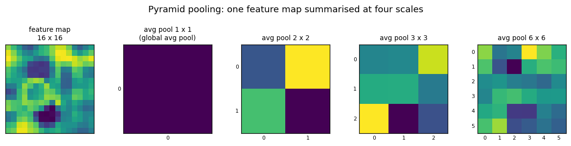
9. DeepLab: atrous (dilated) convolution

Chen et al, TPAMI 2017. DeepLab keeps resolution high with atrous convolution (also called dilated convolution), and aggregates multi-scale context with ASPP (Atrous Spatial Pyramid Pooling), then cleans up boundaries with a fully connected CRF as post-processing.

The idea

A dilated convolution spreads its kernel taps apart by inserting dilation - 1 gaps between them. A \(3\times3\) kernel at dilation \(d\) covers a \((2d+1)\times(2d+1)\) region using only 9 weights and no downsampling:

• more receptive field (it sees wider)

• same resolution (no stride, no pooling, output size unchanged)

• same parameter count (still 9 weights)

The effective kernel size is \(k_{\text{eff}} = d(k-1) + 1\). This is how DeepLab replaces the resolution-destroying pools of a classifier with resolution-preserving context.

# a dilated conv is literally a normal conv on a kernel with zeros inserted between taps
def dilate_kernel(w, d):
    Co, Ci, kh, kw = w.shape
    out = w.new_zeros(Co, Ci, d * (kh - 1) + 1, d * (kw - 1) + 1)
    out[:, :, ::d, ::d] = w
    return out

set_seed()
w = torch.randn(1, 1, 3, 3)
x = torch.randn(1, 1, 17, 17)
for d in [1, 2, 4]:
    keff = d * (3 - 1) + 1
    pad = d * (3 - 1) // 2
    ref = F.conv2d(x, w, dilation=d, padding=pad)              # native dilated conv
    manual = F.conv2d(x, dilate_kernel(w, d), padding=pad)     # same thing, kernel with holes
    assert torch.allclose(ref, manual, atol=1e-5)
    print(f'dilation {d}: 3x3 kernel covers {keff}x{keff}, still 9 weights, '
          f'input {tuple(x.shape[2:])} -> output {tuple(ref.shape[2:])} (unchanged)   '
          f'[matches a holey-kernel plain conv: {torch.allclose(ref, manual, atol=1e-5)}]')
print('\nThe kernel spreads out, the receptive field grows, the resolution and parameter count do not change.')

# show the tap layout: where the 9 weights actually land for each dilation
fig, axes = plt.subplots(1, 3, figsize=(8, 2.8))
for ax, d in zip(axes, [1, 2, 4]):
    keff = d * 2 + 1
    grid = np.zeros((keff, keff))
    grid[::d, ::d] = 1
    ax.imshow(grid, cmap='Oranges', vmin=0, vmax=1)
    ax.set_title(f'dilation {d}\n3x3 taps over {keff}x{keff}')
    ax.set_xticks(range(keff)); ax.set_yticks(range(keff)); ax.tick_params(length=0)
    ax.grid(True, color='0.7', lw=0.5)
plt.suptitle('Where the 9 kernel taps land (orange = a weight, white = a hole)', y=1.06)
plt.tight_layout(); plt.show()

dilation 1: 3x3 kernel covers 3x3, still 9 weights, input (17, 17) -> output (17, 17) (unchanged)   [matches a holey-kernel plain conv: True]
dilation 2: 3x3 kernel covers 5x5, still 9 weights, input (17, 17) -> output (17, 17) (unchanged)   [matches a holey-kernel plain conv: True]
dilation 4: 3x3 kernel covers 9x9, still 9 weights, input (17, 17) -> output (17, 17) (unchanged)   [matches a holey-kernel plain conv: True]

The kernel spreads out, the receptive field grows, the resolution and parameter count do not change.

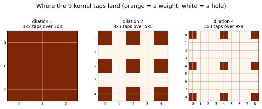
9a. Measuring the receptive field with autograd

We can measure the receptive field instead of computing it by hand. Stack three \(3\times3\) convs at a fixed dilation, put a single 1 in the gradient at the centre of the output, and backpropagate to the input. Every input pixel whose gradient is non-zero is, by definition, in the receptive field of that output pixel. We do this for dilation 1, 2, 4 and overlay the measured extents.

def receptive_field(dilation, n_layers=3, size=49):
    """Backprop a single output pixel to the input; nonzero input-grad = receptive field."""
    torch.manual_seed(0)
    convs = [nn.Conv2d(1, 1, 3, padding=dilation * (3 - 1) // 2, dilation=dilation, bias=False) for _ in range(n_layers)]
    for c in convs:
        nn.init.constant_(c.weight, 0.1)                        # positive weights: no cancellation, clean support
    x = torch.zeros(1, 1, size, size, requires_grad=True)
    h = x
    for c in convs:
        h = c(h)
    h[0, 0, size // 2, size // 2].backward()
    rf = (x.grad[0, 0].abs() > 0).float().numpy()
    return rf, int(rf.sum())

fig, axes = plt.subplots(1, 4, figsize=(11, 2.8))
extents = {}
for ax, d in zip(axes[:3], [1, 2, 4]):
    rf, area = receptive_field(d)
    ys, xs = np.where(rf > 0)
    span = xs.max() - xs.min() + 1
    extents[d] = span
    ax.imshow(rf, cmap='Blues')
    ax.set_title(f'dilation {d}\n{span} x {span} receptive field ({area} px)')
    ax.set_xticks([]); ax.set_yticks([])
axes[3].bar([str(d) for d in [1, 2, 4]], [extents[d] for d in [1, 2, 4]], color='#0077b6', alpha=0.8)
axes[3].set_xlabel('dilation rate'); axes[3].set_ylabel('receptive field width (px)')
axes[3].set_title('3 stacked 3x3 convs'); axes[3].grid(alpha=0.3, axis='y')
plt.suptitle('Receptive field grows with dilation, measured by backprop (resolution never changes)', y=1.06)
plt.tight_layout(); plt.show()
print('Three 3x3 convs: dilation 1 -> 7x7 RF, dilation 2 -> 13x13, dilation 4 -> 25x25. No pooling was used.')

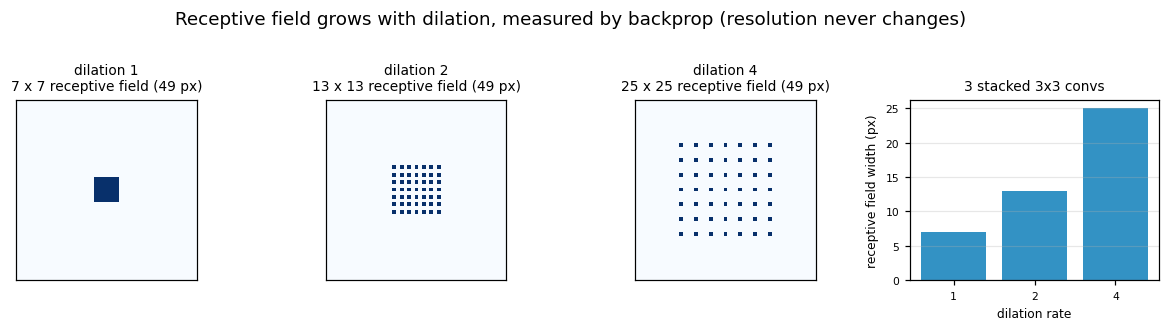
Three 3x3 convs: dilation 1 -> 7x7 RF, dilation 2 -> 13x13, dilation 4 -> 25x25. No pooling was used.

A clarification worth making

The lecture slide (DeepLab, page 56) writes: “atrous convolution = dilated convolution = transpose convolution = fractionally strided convolution”.

The first equality is exactly right, and the last term needs one careful word. For students it is worth separating two genuinely different operations, because they change spatial size in opposite directions:

• Atrous = dilated convolution. Spreads the kernel taps apart to enlarge the receptive field while preserving spatial resolution (output size unchanged, no upsampling). This is section 9.

• Transpose convolution = fractionally strided convolution. Scatters each input over a window to increase spatial resolution (this is the learnable upsampler of section 4).

So “fractionally strided convolution” is a synonym for transpose convolution, not for dilated convolution. A tidy way to keep them apart: a stride-\(s\) transpose conv is equivalent to a normal conv on an input with \(s-1\) zeros inserted between input samples (it dilates the input, growing the output), whereas a dilated conv is a normal conv with \(d-1\) zeros inserted between kernel taps (it dilates the kernel, keeping the output size). Same “insert zeros” trick, different tensor, opposite effect on resolution. The cell below shows both, on the same input, with their shapes.

set_seed()
x = torch.randn(1, 1, 8, 8)
k = torch.randn(1, 1, 3, 3)

dilated = F.conv2d(x, k, dilation=2, padding=2)                # kernel taps spread; resolution preserved
transposed = F.conv_transpose2d(x, k, stride=2, padding=1)     # input scattered; resolution increased

print('same input 1 x 1 x 8 x 8, same 3 x 3 kernel:\n')
print(f'  DILATED  conv2d(dilation=2)          -> {tuple(dilated.shape)}   resolution PRESERVED (8x8), wider receptive field')
print(f'  TRANSPOSE conv_transpose2d(stride=2) -> {tuple(transposed.shape)}   resolution INCREASED (~2x), learnable upsampling')
print('\nThey are different operations. Dilated keeps size; transposed grows it.')

fig, axes = plt.subplots(1, 3, figsize=(8, 2.7))
for ax, im, t in zip(axes, [x, dilated, transposed],
                     ['input 8 x 8', f'dilated conv\n{tuple(dilated.shape[2:])} (same size)',
                      f'transpose conv\n{tuple(transposed.shape[2:])} (bigger)']):
    ax.imshow(im.detach()[0, 0], cmap='RdBu_r'); ax.set_title(t); ax.set_xticks([]); ax.set_yticks([])
plt.tight_layout(); plt.show()

same input 1 x 1 x 8 x 8, same 3 x 3 kernel:

  DILATED  conv2d(dilation=2)          -> (1, 1, 8, 8)   resolution PRESERVED (8x8), wider receptive field
  TRANSPOSE conv_transpose2d(stride=2) -> (1, 1, 15, 15)   resolution INCREASED (~2x), learnable upsampling

They are different operations. Dilated keeps size; transposed grows it.

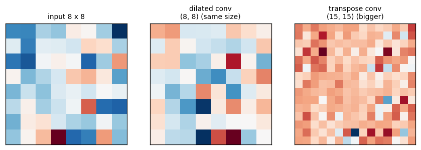
9b. ASPP: Atrous Spatial Pyramid Pooling

ASPP is the atrous analogue of PSPNet’s pyramid: run several dilated convs in parallel at different rates over the same feature map, add a global image-level branch, then concatenate and fuse. Different rates see the object at different scales, all at full resolution. We build a mini ASPP and print the shapes.

class ASPP(nn.Module):
    def __init__(self, in_ch, out_ch=16, rates=(1, 2, 4, 6)):
        super().__init__()
        self.rates = rates
        self.branches = nn.ModuleList()
        for r in rates:
            if r == 1:
                self.branches.append(nn.Conv2d(in_ch, out_ch, 1))                       # 1x1 branch
            else:
                self.branches.append(nn.Conv2d(in_ch, out_ch, 3, padding=r, dilation=r))
        self.image_pool = nn.Sequential(nn.AdaptiveAvgPool2d(1), nn.Conv2d(in_ch, out_ch, 1))  # image-level branch
        self.fuse = nn.Conv2d(out_ch * (len(rates) + 1), out_ch, 1)
    def forward(self, x, verbose=False):
        H, W = x.shape[-2:]
        outs = []
        for r, br in zip(self.rates, self.branches):
            o = br(x); outs.append(o)
            if verbose:
                print(f'  atrous rate {r}: {str(tuple(o.shape)):>22s}   (3x3 covers {r*2+1}x{r*2+1})' if r > 1
                      else f'  1x1 conv    : {str(tuple(o.shape)):>22s}')
        img = F.interpolate(self.image_pool(x), size=(H, W), mode='bilinear', align_corners=False)
        outs.append(img)
        if verbose:
            print(f'  image pool  : {str(tuple(img.shape)):>22s}   (global context, upsampled back)')
        cat = torch.cat(outs, dim=1)
        out = self.fuse(cat)
        if verbose:
            print(f'  concat      : {str(tuple(cat.shape)):>22s}')
            print(f'  fuse 1x1    : {str(tuple(out.shape)):>22s}')
        return out

set_seed()
aspp = ASPP(16)
print('mini ASPP, rates (1, 2, 4, 6) + image-level branch:\n')
_ = aspp(torch.randn(1, 16, 16, 16), verbose=True)
print('\nEvery branch keeps the 16 x 16 resolution. Context is gathered without ever downsampling.')

mini ASPP, rates (1, 2, 4, 6) + image-level branch:

  1x1 conv    :        (1, 16, 16, 16)
  atrous rate 2:        (1, 16, 16, 16)   (3x3 covers 5x5)
  atrous rate 4:        (1, 16, 16, 16)   (3x3 covers 9x9)
  atrous rate 6:        (1, 16, 16, 16)   (3x3 covers 13x13)
  image pool  :        (1, 16, 16, 16)   (global context, upsampled back)
  concat      :        (1, 80, 16, 16)
  fuse 1x1    :        (1, 16, 16, 16)

Every branch keeps the 16 x 16 resolution. Context is gathered without ever downsampling.

Interactive: dilation rate vs receptive field

Slide the dilation rate and the number of stacked layers; read off the effective kernel size, the measured receptive field, and the tap pattern. Larger dilation = wider view, same resolution, same weights.

def dilation_explorer(dilation=2, n_layers=3):
    keff = dilation * 2 + 1
    rf, area = receptive_field(dilation, n_layers=n_layers)
    ys, xs = np.where(rf > 0)
    span = xs.max() - xs.min() + 1
    print(f'3x3 kernel at dilation {dilation}: effective kernel {keff} x {keff}, still 9 weights')
    print(f'{n_layers} stacked layers -> measured receptive field {span} x {span} ({area} pixels), resolution unchanged')
    fig, axes = plt.subplots(1, 2, figsize=(6, 2.9))
    taps = np.zeros((keff, keff)); taps[::dilation, ::dilation] = 1
    axes[0].imshow(taps, cmap='Oranges', vmin=0, vmax=1); axes[0].set_title(f'single-layer taps\n{keff} x {keff}')
    axes[0].set_xticks([]); axes[0].set_yticks([])
    axes[1].imshow(rf, cmap='Blues'); axes[1].set_title(f'{n_layers}-layer receptive field\n{span} x {span}')
    axes[1].set_xticks([]); axes[1].set_yticks([])
    plt.tight_layout(); plt.show()

widgets.interact(dilation_explorer,
                 dilation=widgets.IntSlider(min=1, max=6, step=1, value=2, continuous_update=False),
                 n_layers=widgets.IntSlider(min=1, max=4, step=1, value=3, continuous_update=False));

10. DeepLab v3 and v3+

The family kept improving, and the changes are all about more context and cleaner boundaries:

• v3 adds an image-level feature to ASPP (global average pool, then a \(1\times1\) conv, upsampled back, the branch we already included above), and adds batch normalization throughout for easier training. It also drops the CRF: a strong enough ASPP made the hand-tuned post-processing largely unnecessary.

• v3+ adds a small decoder module to refine results, especially object boundaries (ASPP alone still upsamples by a large factor at the end, which blurs edges), and uses atrous separable convolution: depthwise separable convolutions with atrous rates, which cut computation sharply for the same receptive field.

The throughline of sections 3 to 10: recover spatial detail (FCN skips, SegNet indices, U-Net concat, DeepLab dilation) and gather global context (PSPNet pyramid, DeepLab ASPP). Every architecture is a different mix of those two ingredients.

11. Instance segmentation

Semantic segmentation labels every pixel with a class, but it cannot count. Two disks that touch become one blue blob: same class, no separation. Instance segmentation gives each pixel a class label and an object id, so the two disks become object 1 and object 2.

Our generator already stores instance ids, so we can show the difference directly. Watch what happens where two objects of the same class touch.

# find a validation image where two things of the SAME class touch
def touching_same_class(sem, inst):
    for k in range(1, int(inst.max()) + 1):
        for j in range(k + 1, int(inst.max()) + 1):
            mk = ndi.binary_dilation(inst.numpy() == k)
            if (mk & (inst.numpy() == j)).any() and sem[inst == k][0] == sem[inst == j][0]:
                return True
    return False

idx = next((i for i in range(len(Xva)) if touching_same_class(Sva[i], Iva[i])), 2)
fig, axes = plt.subplots(1, 3, figsize=(7.5, 2.7))
axes[0].imshow(Xva[idx].numpy().transpose(1, 2, 0)); axes[0].set_title('image')
axes[1].imshow(semantic_rgb(Sva[idx].numpy())); axes[1].set_title('semantic\n(touching objects merge)')
axes[2].imshow(instance_rgb(Iva[idx].numpy())); axes[2].set_title('instance\n(each object separated)')
for ax in axes:
    ax.set_xticks([]); ax.set_yticks([])
plt.tight_layout(); plt.show()
print('Semantic segmentation answers "what class is this pixel?". Instance segmentation also answers "which object?".')

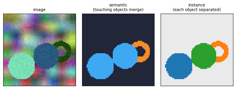
Semantic segmentation answers "what class is this pixel?". Instance segmentation also answers "which object?".

12. Mask R-CNN

He et al, ICCV 2017. The slide’s one-line definition:

Mask R-CNN = Faster R-CNN with an FCN on the RoIs.

Faster R-CNN (lectures 1 to 3) already has, per region proposal (RoI):

• a classification head (what class)

• a box regression head (where, refined)

Mask R-CNN adds, in parallel, a third head:

• a small FCN mask branch that outputs a per-pixel mask for the RoI

Two design choices make it work, and they are the rest of this section:

• RoIAlign instead of RoIPool, so the RoI features line up with the image at the pixel level (section 13)

• the mask head predicts one mask per class with a sigmoid, decoupled from the classification head, trained with binary cross-entropy (section 14)

The mask branch is cheap: it runs on the small, already-cropped RoI feature, not the whole image.

13. RoIAlign vs RoIPool

The slide’s argument:

• Moving a proposal from image space to feature space loses information to quantization (the box coordinates get rounded to the feature grid). RoIPool then quantizes a second time when it snaps its pooling bins to integer cells.

• Why it matters: “one pixel in feature space is equivalent to many pixels on the image”. A backbone with stride 16 means one feature cell covers a \(16\times16\) image patch, so half-a-cell of drift is 8 pixels in the image.

• This barely hurts boxes (a few pixels of slack on a box is fine) but badly hurts masks, which are supposed to be pixel-accurate.

• RoIAlign removes both quantizations: it samples at the exact floating-point locations with bilinear interpolation. This “preserves translation equivariance of masks”: shift the object in the RoI and the mask shifts with it, smoothly.

We implement both from scratch, then cross-check against torchvision.ops with assert torch.allclose(...).

13a. RoIPool: the double quantization

from torchvision.ops import roi_pool, roi_align

def roi_pool_scratch(feat, roi, out=2):
    """feat: (C,H,W). roi: (x1,y1,x2,y2) in feature coords. Quantizes TWICE, exactly like RoIPool."""
    C, H, W = feat.shape
    rnd = lambda v: int(math.floor(float(v) + 0.5))                 # round half away from zero
    x1, y1, x2, y2 = rnd(roi[0]), rnd(roi[1]), rnd(roi[2]), rnd(roi[3])   # quantization 1: image -> feature grid
    rw, rh = max(x2 - x1 + 1, 1), max(y2 - y1 + 1, 1)
    bw, bh = rw / out, rh / out
    o = torch.zeros(C, out, out)
    for ph in range(out):
        for pw in range(out):
            hs = min(max(int(math.floor(ph * bh)) + y1, 0), H)     # quantization 2: bin boundaries -> integers
            he = min(max(int(math.ceil((ph + 1) * bh)) + y1, 0), H)
            ws = min(max(int(math.floor(pw * bw)) + x1, 0), W)
            we = min(max(int(math.ceil((pw + 1) * bw)) + x1, 0), W)
            if he > hs and we > ws:
                o[:, ph, pw] = feat[:, hs:he, ws:we].amax(dim=(1, 2))
    return o

set_seed()
feat = torch.randn(2, 8, 8)
roi = torch.tensor([1.3, 2.7, 6.6, 5.2])                            # deliberately non-integer RoI
mine = roi_pool_scratch(feat, roi, out=2)
boxes = torch.cat([torch.zeros(1), roi])[None]                     # (batch_idx, x1, y1, x2, y2)
ref = roi_pool(feat[None], boxes, output_size=2, spatial_scale=1.0)[0]
assert torch.allclose(mine, ref, atol=1e-5)
print(f'RoIPool from scratch matches torchvision.ops.roi_pool   (max|diff| = {(mine-ref).abs().max():.2e})')
rnd = lambda v: int(math.floor(float(v) + 0.5))
print(f'\nRoI top-left ({roi[0]:.1f}, {roi[1]:.1f}) is rounded to ({rnd(roi[0])}, {rnd(roi[1])}): '
      f'a drift of ({abs(float(roi[0])-rnd(roi[0])):.1f}, {abs(float(roi[1])-rnd(roi[1])):.1f}) feature cells before pooling even starts.')

RoIPool from scratch matches torchvision.ops.roi_pool   (max|diff| = 0.00e+00)

RoI top-left (1.3, 2.7) is rounded to (1, 3): a drift of (0.3, 0.3) feature cells before pooling even starts.

13b. RoIAlign: exact bilinear sampling, no quantization

def bilinear_sample(feat, y, x):
    """Bilinear interpolation at float (y,x), matching torchvision (0 outside [-1,H]x[-1,W])."""
    C, H, W = feat.shape
    if y < -1.0 or y > H or x < -1.0 or x > W:
        return torch.zeros(C)
    y = min(max(y, 0.0), H - 1.0); x = min(max(x, 0.0), W - 1.0)
    y0, x0 = int(math.floor(y)), int(math.floor(x))
    y1, x1 = min(y0 + 1, H - 1), min(x0 + 1, W - 1)
    ly, lx = y - y0, x - x0
    return ((1 - ly) * (1 - lx) * feat[:, y0, x0] + (1 - ly) * lx * feat[:, y0, x1]
            + ly * (1 - lx) * feat[:, y1, x0] + ly * lx * feat[:, y1, x1])

def roi_align_scratch(feat, roi, out=2, sampling_ratio=2):
    """No quantization: divide the FLOAT RoI into bins, sample points per bin bilinearly, average."""
    C = feat.shape[0]
    x1, y1, x2, y2 = [float(v) for v in roi]
    bw, bh = (x2 - x1) / out, (y2 - y1) / out
    o = torch.zeros(C, out, out)
    for ph in range(out):
        for pw in range(out):
            acc = torch.zeros(C)
            for iy in range(sampling_ratio):
                yy = y1 + ph * bh + (iy + 0.5) * bh / sampling_ratio
                for ix in range(sampling_ratio):
                    xx = x1 + pw * bw + (ix + 0.5) * bw / sampling_ratio
                    acc += bilinear_sample(feat, yy, xx)
            o[:, ph, pw] = acc / (sampling_ratio ** 2)
    return o

mine = roi_align_scratch(feat, roi, out=2, sampling_ratio=2)
ref = roi_align(feat[None], boxes, output_size=2, spatial_scale=1.0, sampling_ratio=2, aligned=False)[0]
assert torch.allclose(mine, ref, atol=1e-5)
print(f'RoIAlign from scratch matches torchvision.ops.roi_align   (max|diff| = {(mine-ref).abs().max():.2e})')
print('No coordinate was rounded: the RoI is sampled exactly where it falls.')

RoIAlign from scratch matches torchvision.ops.roi_align   (max|diff| = 2.38e-07)
No coordinate was rounded: the RoI is sampled exactly where it falls.

13c. The sampling grids, overlaid on the feature map

The whole story in one picture. On the same feature map and the same float RoI (dashed white box):

• RoIPool (left): the RoI is snapped to the integer grid (solid box), then split into bins whose edges are snapped again. The red patches are the actual regions max-pooled: notice they do not fill the requested RoI.

• RoIAlign (right): the requested RoI is kept exactly, split into equal bins, and sampled at precise float points (red dots). Nothing is snapped.

out_sz = 2
fig, axes = plt.subplots(1, 2, figsize=(9, 4.2))
x1, y1, x2, y2 = [float(v) for v in roi]

# RoIPool panel
ax = axes[0]
ax.imshow(feat[0], cmap='Greys', alpha=0.85)
ax.add_patch(mpatches.Rectangle((x1 - 0.5, y1 - 0.5), x2 - x1, y2 - y1, fill=False, ec='white', lw=2, ls='--', label='requested RoI'))
qx1, qy1, qx2, qy2 = rnd(x1), rnd(y1), rnd(x2), rnd(y2)
ax.add_patch(mpatches.Rectangle((qx1 - 0.5, qy1 - 0.5), qx2 - qx1 + 1, qy2 - qy1 + 1, fill=False, ec='tab:blue', lw=2, label='quantized RoI'))
rw, rh = max(qx2 - qx1 + 1, 1), max(qy2 - qy1 + 1, 1)
for ph in range(out_sz):
    for pw in range(out_sz):
        hs = int(math.floor(ph * rh / out_sz)) + qy1; he = int(math.ceil((ph + 1) * rh / out_sz)) + qy1
        ws = int(math.floor(pw * rw / out_sz)) + qx1; we = int(math.ceil((pw + 1) * rw / out_sz)) + qx1
        ax.add_patch(mpatches.Rectangle((ws - 0.5, hs - 0.5), we - ws, he - hs, fc='tab:red', alpha=0.25, ec='tab:red'))
ax.set_title('RoIPool: RoI snapped to grid,\nbins snapped again (red = pooled regions)')
ax.legend(loc='upper right', fontsize=6.5)

# RoIAlign panel
ax = axes[1]
ax.imshow(feat[0], cmap='Greys', alpha=0.85)
ax.add_patch(mpatches.Rectangle((x1 - 0.5, y1 - 0.5), x2 - x1, y2 - y1, fill=False, ec='white', lw=2, ls='--', label='requested RoI (kept)'))
bw, bh = (x2 - x1) / out_sz, (y2 - y1) / out_sz
for ph in range(out_sz):
    for pw in range(out_sz):
        ax.add_patch(mpatches.Rectangle((x1 + pw * bw - 0.5, y1 + ph * bh - 0.5), bw, bh, fill=False, ec='tab:green', lw=1))
        for iy in range(2):
            for ix in range(2):
                yy = y1 + ph * bh + (iy + 0.5) * bh / 2
                xx = x1 + pw * bw + (ix + 0.5) * bw / 2
                ax.plot(xx, yy, 'o', color='tab:red', ms=5)
ax.plot([], [], 'o', color='tab:red', ms=5, label='bilinear sample points')
ax.set_title('RoIAlign: RoI kept exactly,\nsampled at precise float points')
ax.legend(loc='upper right', fontsize=6.5)
for ax in axes:
    ax.set_xlim(-0.5, 7.5); ax.set_ylim(7.5, -0.5); ax.set_xticks(range(8)); ax.set_yticks(range(8)); ax.tick_params(length=0); ax.grid(True, color='0.8', lw=0.4)
plt.tight_layout(); plt.show()

drift_x = abs(x1 - qx1) + abs(x2 - qx2)
print(f'RoIPool loses up to ({abs(x1-qx1):.1f} + {abs(x2-qx2):.1f}) = {drift_x:.1f} feature cells of the RoI width to rounding.')
print('With a stride-16 backbone, one feature cell = 16 image pixels, so this is several pixels of image-space drift.')

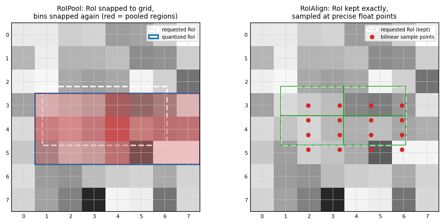
RoIPool loses up to (0.3 + 0.4) = 0.7 feature cells of the RoI width to rounding.
With a stride-16 backbone, one feature cell = 16 image pixels, so this is several pixels of image-space drift.

13d. Why boxes tolerate it but masks do not: translation equivariance

The slide’s key figure: “translation of object in RoI => same translation of mask in RoI”. We slide a sharp feature (a step edge) across the RoI in sub-pixel steps and read out one pooled cell. RoIAlign responds smoothly and monotonically (it tracks the true position). RoIPool responds in stairsteps (it can only see integer positions). For a box that jitter is negligible; for a per-pixel mask it is exactly the error you cannot afford.

shifts = np.linspace(0, 4, 41)
pool_vals, align_vals = [], []
for s in shifts:
    ramp = torch.zeros(1, 8, 8)
    col = np.clip(np.arange(8) - s, 0, None)                        # a moving ramp / edge
    ramp[0] = torch.tensor(np.tile(col, (8, 1)), dtype=torch.float32)
    r = torch.tensor([1.0, 1.0, 6.0, 6.0])
    pool_vals.append(roi_pool_scratch(ramp, r, out=2)[0, 0, 0].item())
    align_vals.append(roi_align_scratch(ramp, r, out=2, sampling_ratio=2)[0, 0, 0].item())

fig, ax = plt.subplots(figsize=(6.5, 3.0))
ax.plot(shifts, pool_vals, 's-', color='tab:red', label='RoIPool (stairsteps: quantized)', ms=3)
ax.plot(shifts, align_vals, 'o-', color='tab:green', label='RoIAlign (smooth: exact sampling)', ms=3)
ax.set_xlabel('sub-pixel shift of the object in the RoI'); ax.set_ylabel('value in one output cell')
ax.set_title('Translation equivariance: RoIAlign tracks sub-pixel motion, RoIPool cannot')
ax.legend(); ax.grid(alpha=0.3)
plt.tight_layout(); plt.show()
print('RoIAlign is smooth in the object position; RoIPool is piecewise-constant. Masks need the smooth one.')

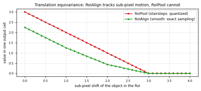
RoIAlign is smooth in the object position; RoIPool is piecewise-constant. Masks need the smooth one.

Interactive: RoIAlign sampling

Move the RoI’s float coordinates and the sampling ratio. The green dots are RoIAlign’s exact sample points; the blue box is where RoIPool would snap the RoI. The printed number is the misalignment RoIPool introduces, in feature cells, that RoIAlign avoids.

def roialign_explorer(x1=1.3, y1=2.7, size=5.0, sampling_ratio=2, out=2):
    x2, y2 = x1 + size, y1 + size
    fig, ax = plt.subplots(figsize=(5.2, 5.0))
    ax.imshow(feat[0], cmap='Greys', alpha=0.85)
    ax.add_patch(mpatches.Rectangle((x1 - 0.5, y1 - 0.5), size, size, fill=False, ec='white', lw=2, ls='--'))
    qx1, qy1, qx2, qy2 = rnd(x1), rnd(y1), rnd(x2), rnd(y2)
    ax.add_patch(mpatches.Rectangle((qx1 - 0.5, qy1 - 0.5), qx2 - qx1 + 1, qy2 - qy1 + 1, fill=False, ec='tab:blue', lw=1.5))
    bw = bh = size / out
    for ph in range(out):
        for pw in range(out):
            for iy in range(sampling_ratio):
                for ix in range(sampling_ratio):
                    yy = y1 + ph * bh + (iy + 0.5) * bh / sampling_ratio
                    xx = x1 + pw * bw + (ix + 0.5) * bw / sampling_ratio
                    ax.plot(xx, yy, 'o', color='tab:green', ms=4)
    ax.set_xlim(-0.5, 7.5); ax.set_ylim(7.5, -0.5); ax.set_xticks(range(8)); ax.set_yticks(range(8))
    ax.tick_params(length=0); ax.grid(True, color='0.8', lw=0.4)
    drift = (abs(x1 - qx1) + abs(y1 - qy1)) / 2
    ax.set_title(f'white dashed = true RoIAlign RoI, blue = RoIPool snap\n'
                 f'{sampling_ratio}x{sampling_ratio} samples/bin | RoIPool corner drift ~ {drift:.2f} feature cells')
    plt.tight_layout(); plt.show()

widgets.interact(roialign_explorer,
                 x1=widgets.FloatSlider(min=0.0, max=3.0, step=0.1, value=1.3, continuous_update=False),
                 y1=widgets.FloatSlider(min=0.0, max=3.0, step=0.1, value=2.7, continuous_update=False),
                 size=widgets.FloatSlider(min=3.0, max=5.5, step=0.1, value=5.0, continuous_update=False),
                 sampling_ratio=widgets.IntSlider(min=1, max=4, step=1, value=2, continuous_update=False));

14. Mask R-CNN: the FCN mask head

The slide:

• an FCN branch generates a mask for each proposal

• the mask is \(28 \times 28\) during training

• at inference it is rescaled to the box and overlaid on the image

The crucial detail is how the mask is scored. The head predicts one \(28\times28\) mask per class (shape \((\text{num classes}, 28, 28)\)) and applies a per-pixel sigmoid, trained with binary cross-entropy on the mask of the ground-truth class only. This decouples mask prediction from class prediction: the classification head decides what the object is, and the corresponding mask channel only has to decide where it is, with no competition between classes inside the mask. (Contrast a softmax over classes per pixel, as in semantic segmentation, where the classes compete.)

We build the tiny head, run it on a \(14\times14\) RoI feature, and check the shapes and the loss.

class MaskHead(nn.Module):
    """A small FCN: four 3x3 convs, one 2x2 transpose conv to double 14->28, a 1x1 conv to per-class masks."""
    def __init__(self, in_ch=16, ncls=NUM_CLASSES, hidden=32):
        super().__init__()
        self.convs = nn.Sequential(*[nn.Sequential(nn.Conv2d(in_ch if i == 0 else hidden, hidden, 3, padding=1),
                                                   nn.ReLU(inplace=True)) for i in range(4)])
        self.deconv = nn.ConvTranspose2d(hidden, hidden, 2, stride=2)      # 14 x 14 -> 28 x 28
        self.predict = nn.Conv2d(hidden, ncls, 1)                          # one mask per class
    def forward(self, x):
        return self.predict(F.relu(self.deconv(self.convs(x))))            # logits, (N, ncls, 28, 28)

set_seed()
head = MaskHead()
roi_feats = torch.randn(4, 16, 14, 14)                                     # 4 proposals, RoIAligned to 14x14
mask_logits = head(roi_feats)
print(f'RoI features        {tuple(roi_feats.shape)}   (4 proposals, 16 channels, 14x14 after RoIAlign)')
print(f'mask head output    {tuple(mask_logits.shape)}   (one 28x28 mask per class, per proposal)')
print(f'\nparameters: {sum(p.numel() for p in head.parameters()):,}')

# per-class sigmoid + binary CE, on the ground-truth class channel only
gt_classes = torch.tensor([1, 2, 1, 2])                                    # class of each proposal
gt_masks = (torch.rand(4, 28, 28) > 0.5).float()                          # toy 28x28 target masks
chosen = mask_logits[torch.arange(4), gt_classes]                         # pick each proposal's GT-class mask
loss = F.binary_cross_entropy_with_logits(chosen, gt_masks)
print(f'\nmask loss = BCE(sigmoid(mask of the GT class), target)  ->  {loss.item():.4f}')
print('Only the ground-truth class channel is supervised. The other class masks get no mask gradient.')
print('This is why the slide says the mask branch is decoupled from classification.')

RoI features        (4, 16, 14, 14)   (4 proposals, 16 channels, 14x14 after RoIAlign)
mask head output    (4, 3, 28, 28)   (one 28x28 mask per class, per proposal)

parameters: 36,611

mask loss = BCE(sigmoid(mask of the GT class), target)  ->  0.6956
Only the ground-truth class channel is supervised. The other class masks get no mask gradient.
This is why the slide says the mask branch is decoupled from classification.

From \(28\times28\) to the image

At inference the per-class \(28\times28\) mask for the predicted class is passed through a sigmoid, thresholded at 0.5, then resized to the proposal box and pasted back. Because RoIAlign kept everything aligned, the small mask lands on the right pixels. Here is the resize-and-paste, on a toy ring-shaped mask.

yy, xx = np.mgrid[0:28, 0:28]
toy = (((yy - 14) ** 2 + (xx - 14) ** 2 <= 12 ** 2) & ((yy - 14) ** 2 + (xx - 14) ** 2 >= 7 ** 2)).astype(np.float32)
box = (10, 8, 46, 52)                                                      # x1,y1,x2,y2 on a 64x64 canvas
bw, bh = box[2] - box[0], box[3] - box[1]
resized = F.interpolate(torch.tensor(toy)[None, None], size=(bh, bw), mode='bilinear', align_corners=False)[0, 0]
canvas = np.zeros((64, 64))
canvas[box[1]:box[3], box[0]:box[2]] = (resized.numpy() > 0.5)

fig, axes = plt.subplots(1, 3, figsize=(7.5, 2.7))
axes[0].imshow(toy, cmap='magma'); axes[0].set_title('28 x 28 mask\n(head output, one class)')
axes[1].imshow(resized, cmap='magma'); axes[1].set_title(f'resized to box\n{bw} x {bh}')
axes[2].imshow(canvas, cmap='magma')
axes[2].add_patch(mpatches.Rectangle((box[0], box[1]), bw, bh, fill=False, ec='cyan', lw=1.5))
axes[2].set_title('pasted onto the image\nat the box location')
for ax in axes:
    ax.set_xticks([]); ax.set_yticks([])
plt.tight_layout(); plt.show()

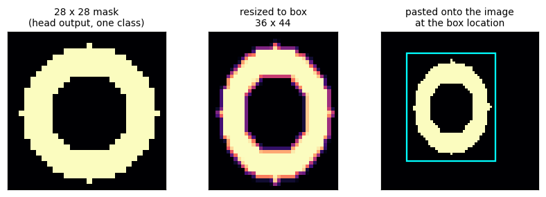
15. Panoptic segmentation

Kirillov et al, CVPR 2019. Panoptic segmentation unifies the two tasks we have kept separate:

• Semantic segmentation handles stuff: amorphous regions (background, sky, road) that have no instances.

• Instance segmentation handles things: countable objects (our rings and disks) that have instances.

• Panoptic segmentation assigns every pixel exactly one semantic label and, if it is a thing, one instance id. No pixel is left unlabelled (unlike instance segmentation) and things are still counted (unlike semantic segmentation). Every pixel belongs to exactly one segment; segments never overlap.

A possible architecture

The slide sketches a shared design:

• a shared backbone

• an instance branch (a Mask R-CNN style head: classification, box, mask)

• a semantic branch (an FCN style head producing per-pixel class scores, including stuff classes)

• a fusion step resolves overlaps into one label per pixel

The combined loss simply adds the two branches:

\[\mathcal{L} = \lambda_i\,(\mathcal{L}_{cls} + \mathcal{L}_{bbox} + \mathcal{L}_{mask}) + \lambda_s\,\mathcal{L}_{s}\]

where \(\mathcal{L}_{cls}, \mathcal{L}_{bbox}, \mathcal{L}_{mask}\) are the instance branch losses and \(\mathcal{L}_s\) is the semantic branch’s pixel-wise cross-entropy.

We build a panoptic label for one of our images by fusing the semantic map (for stuff) with the instance map (for things), exactly as such an architecture would at the end.

def build_panoptic(sem, inst):
    """Fuse a semantic map (stuff) and an instance map (things) into (class, instance_id) per pixel."""
    H, W = sem.shape
    pan_class = sem.copy()
    pan_inst = inst.copy()                                       # 0 for stuff, 1..K for things
    segments = []
    for c in STUFF_CLASSES:                                      # stuff: one segment per class, instance id 0
        if (sem == c).any():
            segments.append(('stuff', c, 0, int((sem == c).sum())))
    for k in range(1, int(inst.max()) + 1):                      # things: one segment per instance
        m = inst == k
        if m.any():
            segments.append(('thing', int(sem[m][0]), k, int(m.sum())))
    return pan_class, pan_inst, segments

sem0, inst0 = Sva[3].numpy(), Iva[3].numpy()
pc, pi, segs = build_panoptic(sem0, inst0)
print('panoptic segments (kind, class, instance_id, area):')
for kind, c, iid, area in segs:
    print(f'  {kind:5s}  class={CLASS_NAMES[c]:11s} instance={iid}  area={area} px')

fig, axes = plt.subplots(1, 4, figsize=(9.5, 2.7))
axes[0].imshow(Xva[3].numpy().transpose(1, 2, 0)); axes[0].set_title('image')
axes[1].imshow(semantic_rgb(sem0)); axes[1].set_title('semantic (stuff + things)')
axes[2].imshow(instance_rgb(inst0)); axes[2].set_title('instance (things only)')
axes[3].imshow(panoptic_rgb(sem0, inst0)); axes[3].set_title('panoptic (fused)')
for ax in axes:
    ax.set_xticks([]); ax.set_yticks([])
plt.tight_layout(); plt.show()

panoptic segments (kind, class, instance_id, area):
  stuff  class=background  instance=0  area=3207 px
  thing  class=ring        instance=1  area=150 px
  thing  class=disk        instance=2  area=475 px
  thing  class=ring        instance=3  area=264 px

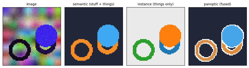
16. Panoptic quality (PQ)

Why a new metric

The slide asks why we cannot reuse the old metrics:

• semantic segmentation uses IoU / pixel accuracy (no notion of instances)

• instance segmentation uses average precision over IoU thresholds (no notion of stuff, needs confidence scores)

• gluing them together is asymmetric: classes with instance annotations and classes without would be scored on different footings

The definition

Match each predicted segment to a ground-truth segment. A pair is a true positive if \(\text{IoU} > 0.5\); because that threshold exceeds one half, each segment can match at most one other, so the matching is unique and unambiguous. Unmatched predictions are false positives, unmatched ground-truth segments are false negatives. Then

\[PQ = \frac{\sum_{(p,g)\in TP} \text{IoU}(p,g)}{|TP| + \tfrac{1}{2}|FP| + \tfrac{1}{2}|FN|} = \underbrace{\frac{\sum_{(p,g)\in TP}\text{IoU}(p,g)}{|TP|}}_{\text{SQ (segmentation quality)}} \;\times\; \underbrace{\frac{|TP|}{|TP| + \tfrac{1}{2}|FP| + \tfrac{1}{2}|FN|}}_{\text{RQ (recognition quality)}}\]

The factorisation is clean: SQ is the average IoU of the segments you got right (how well-shaped are the hits), RQ is an F1-like detection score (did you find the right set of objects at all). We build PQ from scratch on a hand-made example with known TP/FP/FN and check the factorisation numerically.

def iou_mask(a, b):
    inter = (a & b).sum()
    union = (a | b).sum()
    return inter / union if union > 0 else 0.0

def panoptic_quality(gt_masks, pred_masks, thr=0.5):
    """Greedy IoU>0.5 matching (unique because thr > 0.5). Returns PQ, SQ, RQ and the counts."""
    matched_pred, matched_gt, iou_sum = set(), set(), 0.0
    pairs = []
    for gi, g in enumerate(gt_masks):
        for pi, p in enumerate(pred_masks):
            if pi in matched_pred:
                continue
            v = iou_mask(g, p)
            if v > thr:
                matched_gt.add(gi); matched_pred.add(pi); iou_sum += v
                pairs.append((gi, pi, v)); break
    TP, FP, FN = len(matched_gt), len(pred_masks) - len(matched_pred), len(gt_masks) - len(matched_gt)
    SQ = iou_sum / TP if TP else 0.0
    RQ = TP / (TP + 0.5 * FP + 0.5 * FN) if (TP + FP + FN) else 0.0
    PQ = iou_sum / (TP + 0.5 * FP + 0.5 * FN) if (TP + FP + FN) else 0.0
    return dict(PQ=PQ, SQ=SQ, RQ=RQ, TP=TP, FP=FP, FN=FN, pairs=pairs)

# a hand-built example on a 12 x 12 grid: 3 GT segments; prediction has 2 hits, 1 spurious, 1 miss
def block(y0, y1, x0, x1, H=12, W=12):
    m = np.zeros((H, W), bool); m[y0:y1, x0:x1] = True; return m

gt_masks = [block(0, 6, 0, 6), block(0, 5, 7, 12), block(7, 12, 0, 5)]
pred_masks = [block(0, 6, 0, 5),        # strong overlap with gt0  -> TP
              block(1, 5, 7, 12),       # strong overlap with gt1  -> TP
              block(7, 12, 7, 12)]      # overlaps nothing (gt2 missed) -> FP and FN

r = panoptic_quality(gt_masks, pred_masks)
for gi, pi, v in r['pairs']:
    print(f'  matched gt{gi} <-> pred{pi}, IoU = {v:.3f}')
print(f'\nTP={r["TP"]}  FP={r["FP"]}  FN={r["FN"]}')
print(f'SQ = {r["SQ"]:.4f}   RQ = {r["RQ"]:.4f}   PQ = {r["PQ"]:.4f}')
print(f'SQ x RQ = {r["SQ"] * r["RQ"]:.4f}')
assert abs(r['PQ'] - r['SQ'] * r['RQ']) < 1e-9
print('assert PQ == SQ x RQ   PASSED')

  matched gt0 <-> pred0, IoU = 0.833
  matched gt1 <-> pred1, IoU = 0.800

TP=2  FP=1  FN=1
SQ = 0.8167   RQ = 0.6667   PQ = 0.5444
SQ x RQ = 0.5444
assert PQ == SQ x RQ   PASSED

The example, drawn, and PQ = SQ x RQ as bars

fig, axes = plt.subplots(1, 3, figsize=(10, 3.0))
gt_lab = np.zeros((12, 12)); pred_lab = np.zeros((12, 12))
for i, m in enumerate(gt_masks):
    gt_lab[m] = i + 1
for i, m in enumerate(pred_masks):
    pred_lab[m] = i + 1
axes[0].imshow(gt_lab, cmap='tab10', vmin=0, vmax=10); axes[0].set_title('ground truth\n3 segments')
axes[1].imshow(pred_lab, cmap='tab10', vmin=0, vmax=10); axes[1].set_title('prediction\n2 hits, 1 spurious')
for ax in axes[:2]:
    ax.set_xticks([]); ax.set_yticks([])
bars = axes[2].bar(['SQ', 'RQ', 'PQ', 'SQ x RQ'], [r['SQ'], r['RQ'], r['PQ'], r['SQ'] * r['RQ']],
                   color=['#8ecae6', '#ffb703', '#fb8500', '#023047'], alpha=0.9)
for b, v in zip(bars, [r['SQ'], r['RQ'], r['PQ'], r['SQ'] * r['RQ']]):
    axes[2].text(b.get_x() + b.get_width() / 2, v + 0.01, f'{v:.3f}', ha='center', fontsize=8)
axes[2].set_ylim(0, 1); axes[2].set_title('PQ factorises as SQ x RQ'); axes[2].grid(alpha=0.3, axis='y')
plt.tight_layout(); plt.show()

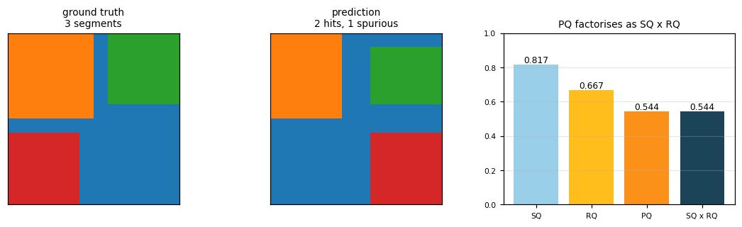
Interactive: the PQ explorer

Set the number of true positives, false positives and false negatives, and the average IoU of the matched segments (that average is SQ). Watch PQ, SQ and RQ update, and confirm the identity \(PQ = SQ \times RQ\) holds for every setting. Notice how FP and FN each cost half a unit in the denominator, and how a high SQ cannot rescue a low RQ.

def pq_explorer(TP=2, FP=1, FN=1, mean_match_IoU=0.80):
    denom = TP + 0.5 * FP + 0.5 * FN
    if TP == 0 or denom == 0:
        print('need at least one true positive for SQ to be defined'); return
    SQ = mean_match_IoU
    RQ = TP / denom
    PQ = (mean_match_IoU * TP) / denom
    print(f'SQ = mean matched IoU           = {SQ:.4f}')
    print(f'RQ = TP / (TP + 0.5FP + 0.5FN)  = {TP} / {denom:.1f} = {RQ:.4f}')
    print(f'PQ = SQ x RQ                    = {PQ:.4f}   (check: {SQ * RQ:.4f})')
    assert abs(PQ - SQ * RQ) < 1e-9
    fig, ax = plt.subplots(figsize=(5.2, 2.8))
    bars = ax.bar(['SQ', 'RQ', 'PQ'], [SQ, RQ, PQ], color=['#8ecae6', '#ffb703', '#fb8500'], alpha=0.9)
    for b, v in zip(bars, [SQ, RQ, PQ]):
        ax.text(b.get_x() + b.get_width() / 2, v + 0.01, f'{v:.3f}', ha='center', fontsize=9)
    ax.set_ylim(0, 1); ax.set_title(f'TP={TP} FP={FP} FN={FN}, mean matched IoU={mean_match_IoU:.2f}')
    ax.grid(alpha=0.3, axis='y')
    plt.tight_layout(); plt.show()

widgets.interact(pq_explorer,
                 TP=widgets.IntSlider(min=0, max=10, step=1, value=2, continuous_update=False),
                 FP=widgets.IntSlider(min=0, max=10, step=1, value=1, continuous_update=False),
                 FN=widgets.IntSlider(min=0, max=10, step=1, value=1, continuous_update=False),
                 mean_match_IoU=widgets.FloatSlider(min=0.5, max=1.0, step=0.02, value=0.80, continuous_update=False));

17. From evaluation metric to loss function: IoU, Dice and Dice loss

The slide closes the loop: the metrics we evaluate with can, with care, become the loss we train with.

• IoU (Jaccard): for a predicted region \(A\) and ground truth \(B\), \(\displaystyle \text{IoU} = \frac{|A \cap B|}{|A \cup B|}\)

• mean IoU: \(\displaystyle \text{mIoU} = \frac{1}{N}\sum_{i=1}^{N}\text{IoU}_i\), averaged over the \(N\) classes (our training metric from section 7c)

• Dice coefficient: \(\displaystyle \text{Dice} = \frac{2|A \cap B|}{|A| + |B|}\)

IoU and Dice measure the same thing and are monotonically related: \(\text{IoU} = \dfrac{\text{Dice}}{2 - \text{Dice}}\). So ranking by one equals ranking by the other; they only differ in how they scale the score.

Why not train on IoU directly? The hard intersection and union use non-differentiable counting (argmax). The fix is the soft / differentiable Dice loss: feed in probabilities \(p \in [0,1]\) instead of hard labels, so \(|A \cap B| \to \sum_i p_i g_i\) and \(|A| \to \sum_i p_i\):

\[\text{DiceLoss}(g, p) = 1 - \frac{2\sum_i p_i g_i + \epsilon}{\sum_i p_i + \sum_i g_i + \epsilon}\]

The \(\epsilon\) is for numerical stability (and defines the loss when a class is absent). We implement all of these from scratch and verify the IoU-Dice relationship.

def iou_score(pred_mask, gt_mask):
    inter = (pred_mask & gt_mask).sum().float()
    union = (pred_mask | gt_mask).sum().float()
    return (inter / union).item() if union > 0 else 1.0

def dice_coeff(pred_mask, gt_mask):
    inter = (pred_mask & gt_mask).sum().float()
    return (2 * inter / (pred_mask.sum() + gt_mask.sum()).float()).item()

def soft_dice_loss(probs, target_onehot, eps=1.0):
    """probs, target_onehot: (N, C, H, W). Mean over classes of the soft Dice loss."""
    dims = (0, 2, 3)
    inter = (probs * target_onehot).sum(dims)
    denom = probs.sum(dims) + target_onehot.sum(dims)
    dice = (2 * inter + eps) / (denom + eps)
    return (1 - dice).mean()

# IoU and Dice on a real prediction from our trained U-Net (foreground vs background)
with torch.no_grad():
    pred = unet_skip(Xva[:16].to(device)).argmax(1).cpu()
pm = (pred > 0); gm = (Sva[:16] > 0)                              # foreground masks
print(f'foreground IoU  = {iou_score(pm, gm):.4f}')
print(f'foreground Dice = {dice_coeff(pm, gm):.4f}')
iou = iou_score(pm, gm); dice = dice_coeff(pm, gm)
print(f'\ncheck IoU = Dice / (2 - Dice): {dice/(2-dice):.4f} vs measured IoU {iou:.4f}   match={abs(iou - dice/(2-dice)) < 1e-4}')

# soft dice loss is differentiable: confirm it produces a gradient
set_seed()
logits = torch.randn(2, NUM_CLASSES, 16, 16, requires_grad=True)
target = torch.randint(0, NUM_CLASSES, (2, 16, 16))
oh = F.one_hot(target, NUM_CLASSES).permute(0, 3, 1, 2).float()
loss = soft_dice_loss(F.softmax(logits, 1), oh)
loss.backward()
print(f'\nsoft Dice loss = {loss.item():.4f}, gradient exists: {logits.grad is not None} '
      f'(max |grad| = {logits.grad.abs().max():.3e})  -> usable for training')

foreground IoU  = 0.9304
foreground Dice = 0.9639

check IoU = Dice / (2 - Dice): 0.9304 vs measured IoU 0.9304   match=True

soft Dice loss = 0.6572, gradient exists: True (max |grad| = 5.135e-04)  -> usable for training

Why Dice tolerates class imbalance better than plain cross-entropy

Pixel-wise cross-entropy averages over all pixels, so a rare foreground class contributes little and the network can drive the loss down by getting the abundant background right. Dice normalises by the sizes of the regions themselves, so a small object counts as much as a large one.

We make this concrete: fix a foreground fraction \(f\), let the predictor assign probability \(p\) to the true-foreground pixels (and near-zero to background), and plot both losses against \(p\). The cross-entropy curves flatten as \(f\) shrinks (its foreground signal fades), while the Dice curve stays essentially the same regardless of \(f\).

def losses_for(f, p, n=40, eps=1.0):
    N = n * n
    g = torch.zeros(N); g[:int(f * N)] = 1.0
    pr = torch.where(g > 0, torch.tensor(float(p)), torch.tensor(0.01))
    bce = F.binary_cross_entropy(pr.clamp(1e-4, 1 - 1e-4), g).item()
    dice = (1 - (2 * (pr * g).sum() + eps) / (pr.sum() + g.sum() + eps)).item()
    return bce, dice

ps = np.linspace(0.02, 0.98, 40)
fig, axes = plt.subplots(1, 2, figsize=(9.5, 3.2))
for f, col in [(0.5, '#023047'), (0.1, '#0077b6'), (0.02, '#8ecae6')]:
    axes[0].plot(ps, [losses_for(f, p)[0] for p in ps], color=col, label=f'f = {f}')
    axes[1].plot(ps, [losses_for(f, p)[1] for p in ps], color=col, label=f'f = {f}')
axes[0].set_title('cross-entropy loss vs P(foreground)\n(collapses as foreground gets rarer)')
axes[1].set_title('Dice loss vs P(foreground)\n(nearly invariant to foreground fraction)')
for ax in axes:
    ax.set_xlabel('predicted foreground probability p'); ax.set_ylabel('loss'); ax.legend(); ax.grid(alpha=0.3)
plt.tight_layout(); plt.show()
print('CE lets a rare class be ignored; Dice keeps caring about it. This is why segmentation often uses Dice,')
print('or a compound loss (CE + Dice), especially in imbalanced domains like medical imaging.')

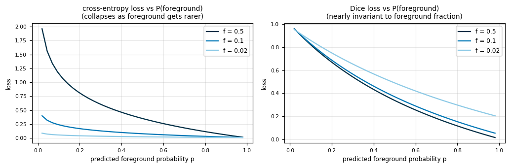
CE lets a rare class be ignored; Dice keeps caring about it. This is why segmentation often uses Dice,
or a compound loss (CE + Dice), especially in imbalanced domains like medical imaging.

Interactive: Dice vs cross-entropy

Set the foreground fraction and the predicted foreground probability, and compare the two losses directly. Push the fraction down to 0.02 (a small object) and see cross-entropy report a tiny loss even for a mediocre probability, while Dice stays informative.

def dice_ce_explorer(foreground_fraction=0.10, predicted_probability=0.50):
    bce, dice = losses_for(foreground_fraction, predicted_probability)
    print(f'foreground fraction f = {foreground_fraction:.2f}, predicted P(foreground) = {predicted_probability:.2f}')
    print(f'  cross-entropy loss = {bce:.4f}')
    print(f'  Dice loss          = {dice:.4f}')
    fig, ax = plt.subplots(figsize=(4.6, 2.8))
    bars = ax.bar(['cross-entropy', 'Dice'], [bce, dice], color=['#e63946', '#0077b6'], alpha=0.85)
    for b, v in zip(bars, [bce, dice]):
        ax.text(b.get_x() + b.get_width() / 2, v + 0.005, f'{v:.3f}', ha='center', fontsize=9)
    ax.set_ylabel('loss'); ax.set_title('same prediction, two losses'); ax.grid(alpha=0.3, axis='y')
    plt.tight_layout(); plt.show()

widgets.interact(dice_ce_explorer,
                 foreground_fraction=widgets.FloatSlider(min=0.02, max=0.5, step=0.02, value=0.10, continuous_update=False),
                 predicted_probability=widgets.FloatSlider(min=0.05, max=0.95, step=0.05, value=0.50, continuous_update=False));

18. A taxonomy of segmentation losses

The slide ends with a map of the loss landscape (Azad et al, “Loss Functions in the Era of Semantic Segmentation: A Survey and Outlook”, 2023). The four families:

Family	Based on	Examples	When it helps
Distribution-based	matching per-pixel class distributions	cross-entropy, weighted CE, focal loss, TopK	the default; focal down-weights easy pixels
Region-based	overlap of predicted and true regions	Dice, IoU / Jaccard, Tversky, Lovasz	class imbalance, when overlap is the metric
Boundary-based	distance between predicted and true boundaries	boundary loss, Hausdorff distance loss	thin structures, precise edges
Compound	weighted sums of the above	CE + Dice, Combo, unified focal	robustness, best of several worlds

Two loss ideas the lecture flagged elsewhere fit right in here:

• U-Net’s weighted cross-entropy (section 7): a distribution-based loss with a per-pixel weight map that up-weights the thin gaps between touching cells, to force the network to separate them. It is exactly the “weighted loss to penalize pixels closer to edges” from the U-Net slide.

• Soft Dice (section 17): the canonical region-based loss.

There is no universally best loss: the right choice depends on the class balance, whether boundaries or regions matter more, and the evaluation metric you are ultimately judged on.

Key takeaways

The semantic architectures at a glance

Model	Upsampling method	Skip / fusion type	Context module	Key idea
FCN	transpose conv (learned)	sum of score maps (32s/16s/8s)	none	make a classifier fully convolutional, then upsample
SegNet	max-unpool via pooling indices	pooling indices (not features)	none	remember where the maxima were; cheap, sharp boundaries
U-Net	transpose conv (learned)	concatenate encoder features	none (depth of the U)	carry fine detail across the U; built for thin structures
PSPNet	bilinear	concat pyramid levels	pyramid pooling (1,2,3,6)	pool at multiple scales for global context
DeepLab	bilinear (+ v3+ decoder)	v3+ decoder skip	ASPP (atrous, multi-rate)	dilate the kernel: more context, full resolution

The three segmentation tasks

Task	Question per pixel	Stuff	Things counted	Metric
Semantic	which class?	labelled	no	IoU / mIoU, pixel accuracy
Instance	which object (and class)?	ignored	yes	AP over IoU thresholds
Panoptic	which class, and which object?	labelled	yes	PQ = SQ x RQ

The two recurring problems, and every architecture’s answer

• Recover spatial detail lost to downsampling: FCN skip sums, SegNet pooling indices, U-Net concatenation, DeepLab dilation (avoid losing it in the first place).

• Gather global context: PSPNet pyramid pooling, DeepLab ASPP, and, for instance-level reasoning, Mask R-CNN’s per-RoI heads with RoIAlign.

What we verified, not just asserted

• from-scratch transpose conv matches nn.ConvTranspose1d / 2d (1D and 2D, allclose)

• from-scratch RoIPool / RoIAlign match torchvision.ops (allclose)

• the tiny U-Net genuinely learned (val mIoU improved from near zero to a healthy value), and the skip-connection ablation produced a real, measured gap, larger at boundaries

• \(PQ = SQ \times RQ\) holds numerically, and \(\text{IoU} = \text{Dice}/(2 - \text{Dice})\)

Exercises

1. FCN-16s vs FCN-8s, measured. The FCN class in section 5 already supports all three modes. Give it the same \(1\times1\)-conv-to-NUM_CLASSES output head, train each mode briefly on our dataset (reuse the train_unet loop with a small step budget), and plot boundary mIoU against the number of skips fused. Does adding the pool3 skip help boundaries as the detail-ceiling argument predicts?

2. A compound loss. Combine the two losses you built: \(\mathcal{L} = \text{CE} + \lambda\,\text{DiceLoss}\). Retrain the tiny U-Net for a few values of \(\lambda \in \{0, 0.5, 1, 2\}\) and report the ring-class IoU (the rare, thin class). At what \(\lambda\) does the region-based term start to help the minority class, and does it ever hurt the majority class?

3. A weighted-loss boundary map (U-Net’s trick). For each training mask, compute a per-pixel weight that is high in the thin gap between two touching instances of the same class (hint: scipy.ndimage.distance_transform_edt to the two nearest instances, as in the U-Net paper). Pass it as the weight/per-pixel factor of a weighted cross-entropy and check whether touching disks separate more cleanly than under plain CE.

4. Panoptic quality on your own predictions. Turn the trained U-Net’s semantic output into instances by connected components (scipy.ndimage.label) on the foreground, build predicted panoptic segments, and run the panoptic_quality function against the ground-truth segments. Break the score down into SQ and RQ: is your network losing more to segmentation quality (shape) or recognition quality (missed or spurious objects)?