📺 Lecture video  |  📄 Slides

Watch on YouTube

Week 2, Lecture 2: From Edges to Blobs and Corners

NPTEL Deep Learning for Computer Vision | Prof. Vineeth N Balasubramanian, IIT Hyderabad

Companion notebook for §2.2 Blob and Corner Detection.

What you will learn

• Detect blobs with the Laplacian of Gaussian.

• Read the local autocorrelation surface and classify a window as flat, edge or corner.

• Use the eigenvalues of the second-moment matrix to make that classification precise.

• Implement the Harris corner detector and compare the common cornerness measures.

• Test how the detector behaves under rotation and scale.

Contents

1. From edge pixels to line segments

2. The Laplacian of Gaussian

3. LoG as a blob detector

4. Flat, edge, corner: the autocorrelation surface

5. Eigenvalues classify the window

6. The Harris corner detector

7. Cornerness measures and variants

8. Properties: rotation and scale

How to run Runs on Colab or a local Jupyter, CPU only. Every image is bundled with scikit-image, so nothing is downloaded. Run the setup cell first, then go top to bottom.

Review

The previous lecture produced Canny edges. This lecture moves to second-order structure (the Laplacian of Gaussian and blobs) and to corners (the Harris detector).

One tool recurs throughout: the eigen-analysis of a local \(2 \times 2\) matrix. We meet it three times, for the orientation of a line, the shape of a blob, and the cornerness of a window. Its eigenvalues describe how strongly a quantity varies along two orthogonal directions.

Setup

Everything uses images bundled with scikit-image, so the notebook runs offline. The helper second_moment_eigs builds the per-pixel second moment matrix and its eigenvalues once, since sections 5 to 8 all reuse it.

%matplotlib inline
import numpy as np
import matplotlib.pyplot as plt
from scipy import ndimage as ndi
from skimage import data, util, color
from skimage.transform import rotate
from skimage.feature import blob_log, corner_harris, corner_peaks, peak_local_max

np.random.seed(0)
plt.rcParams['figure.figsize'] = (10, 4)
plt.rcParams['image.cmap']     = 'gray'
plt.rcParams['figure.dpi']     = 85

def load_gray(image):
    return color.rgb2gray(image) if image.ndim == 3 else util.img_as_float(image)

def show(ax, im, title='', cmap='gray'):
    ax.imshow(im, cmap=cmap); ax.set_title(title); ax.axis('off')

def second_moment_eigs(Ix, Iy, sigma_w):
    # Gaussian-weighted second moment matrix entries a, b, c and its eigenvalues lam1 >= lam2
    a = ndi.gaussian_filter(Ix * Ix, sigma_w)
    b = ndi.gaussian_filter(Ix * Iy, sigma_w)
    c = ndi.gaussian_filter(Iy * Iy, sigma_w)
    tmp  = np.sqrt(((a - c) / 2)**2 + b**2)
    lam1 = (a + c) / 2 + tmp
    lam2 = (a + c) / 2 - tmp
    return a, b, c, lam1, lam2

1. From edge pixels to line segments

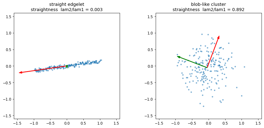
One use of Canny edges is grouping connected edge pixels into straight line segments. Given the pixel coordinates \((x, y)\) of an edgelet with mean \((\mu_x, \mu_y)\), form the second moment matrix

\[\begin{split} M = \begin{bmatrix} \sum (x - \mu_x)^2 & \sum (x - \mu_x)(y - \mu_y) \\ \sum (x - \mu_x)(y - \mu_y) & \sum (y - \mu_y)^2 \end{bmatrix}, \qquad [\,\mathbf{v}, \lambda\,] = \mathrm{eig}(M). \end{split}\]

The eigenvectors give the principal axes of the point cloud and the eigenvalues give its spread along them:

• orientation \(\;\theta = \tan^{-1}(\mathbf{v}_1)\;\) from the larger eigenvector

• straightness \(\;\lambda_2 / \lambda_1\;\) (near \(0\) means a thin, straight segment; near \(1\) means a round cluster)

def moment_matrix(pts):
    d = pts - pts.mean(0)
    M = (d.T @ d) / len(pts)
    lam, V = np.linalg.eigh(M)              # ascending
    return M, lam[::-1], V[:, ::-1]         # return larger eigenvalue first

t = np.linspace(-1, 1, 200)
sets = {
    'straight edgelet':  np.c_[t, 0.15*t] + 0.03*np.random.randn(200, 2),
    'blob-like cluster': 0.40*np.random.randn(200, 2),
}

fig, ax = plt.subplots(1, 2, figsize=(11, 5))
for a, (name, pts) in zip(ax, sets.items()):
    M, lam, V = moment_matrix(pts)
    mu = pts.mean(0)
    a.scatter(pts[:, 0], pts[:, 1], s=8, alpha=0.5)
    for k in range(2):                      # principal axes scaled by sqrt(eigenvalue)
        vec = V[:, k] * np.sqrt(lam[k]) * 2.5
        a.arrow(mu[0], mu[1], vec[0], vec[1], color='r' if k == 0 else 'g',
                width=0.012, head_width=0.06, length_includes_head=True)
    a.set_title(f'{name}\nstraightness  lam2/lam1 = {lam[1]/lam[0]:.3f}')
    a.set_aspect('equal'); a.set_xlim(-1.6, 1.6); a.set_ylim(-1.6, 1.6)
plt.tight_layout(); plt.show()

2. The Laplacian of Gaussian

The orientation-free second derivative is the Laplacian

\[ \nabla^2 f = \frac{\partial^2 f}{\partial x^2} + \frac{\partial^2 f}{\partial y^2}. \]

Each second partial has a discrete form

\[ \frac{\partial^2 f}{\partial x^2} = f(x{+}1, y) + f(x{-}1, y) - 2 f(x, y), \qquad \frac{\partial^2 f}{\partial y^2} = f(x, y{+}1) + f(x, y{-}1) - 2 f(x, y), \]

and their sum collapses to a single \(3 \times 3\) kernel

\[\begin{split} \nabla^2 f = f(x{+}1, y) + f(x{-}1, y) + f(x, y{+}1) + f(x, y{-}1) - 4 f(x, y) \;\;\Longrightarrow\;\; \begin{bmatrix} 0 & 1 & 0 \\ 1 & -4 & 1 \\ 0 & 1 & 0 \end{bmatrix}. \end{split}\]

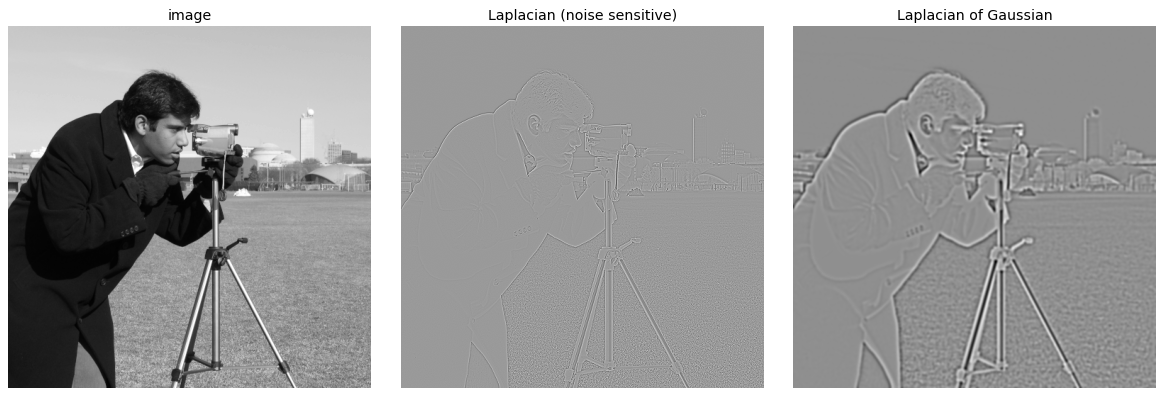
The bare Laplacian amplifies noise, so we smooth with a Gaussian first. The combined operator is the Laplacian of Gaussian (LoG), \(\nabla^2 (f * g)\).

cam = load_gray(data.camera())
laplacian_k = np.array([[0, 1, 0], [1, -4, 1], [0, 1, 0]], float)

lap = ndi.convolve(cam, laplacian_k)        # bare Laplacian
log = ndi.gaussian_laplace(cam, sigma=2)    # Laplacian of Gaussian

fig, ax = plt.subplots(1, 3, figsize=(14, 4.6))
show(ax[0], cam, 'image')
show(ax[1], lap, 'Laplacian (noise sensitive)')
show(ax[2], log, 'Laplacian of Gaussian')
plt.tight_layout(); plt.show()

3. LoG as a blob detector

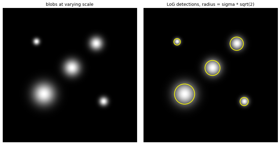
The LoG kernel is circularly symmetric, so convolution measures how well a local region matches a radially symmetric bump. A blob of radius \(r\) produces the strongest response at the matching scale

\[ \sigma \approx \frac{r}{\sqrt{2}}, \qquad \text{detected radius} = \sigma \sqrt{2}. \]

Searching across scales \(\sigma\) and keeping the response peak performs automatic scale selection. Below, blobs of different sizes are each found at their own scale.

H = W = 360
yy, xx = np.mgrid[0:H, 0:W]
planted = [(90, 90, 6), (95, 250, 12), (160, 185, 15), (230, 110, 20), (250, 270, 8)]

blobs = np.zeros((H, W))
for cy, cx, s in planted:
    blobs += np.exp(-((yy - cy)**2 + (xx - cx)**2) / (2 * s**2))
blobs /= blobs.max()

# blob_log searches scales and returns (y, x, sigma) per detection
detections = blob_log(blobs, min_sigma=3, max_sigma=24, num_sigma=14, threshold=0.06)

fig, ax = plt.subplots(1, 2, figsize=(11, 5.5))
show(ax[0], blobs, 'blobs at varying scale')
show(ax[1], blobs, 'LoG detections, radius = sigma * sqrt(2)')
for y, x, s in detections:
    ax[1].add_patch(plt.Circle((x, y), s * np.sqrt(2), color='yellow', fill=False, lw=1.8))
plt.tight_layout(); plt.show()

4. Flat, edge, corner: the autocorrelation surface

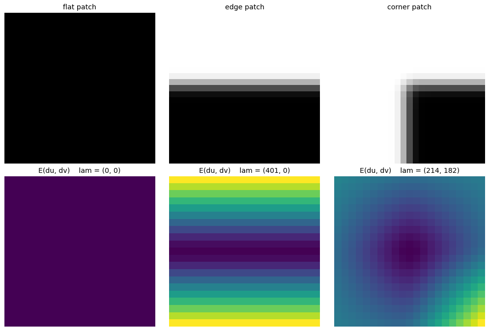
To find corners, ask how a small window changes when shifted by \(\Delta u\). The autocorrelation is the weighted sum of squared differences

\[ E_{AC}(\Delta u) = \sum_{x, y} w(x, y) \, \big[\, I(p + \Delta u) - I(p) \,\big]^2 . \]

A first-order Taylor expansion \(I(p + \Delta u) \approx I(p) + \nabla I(p)\, \Delta u\) turns this into a quadratic form

\[\begin{split} E_{AC}(\Delta u) \approx \Delta u^\top A \, \Delta u, \qquad A = w * \begin{bmatrix} I_x^2 & I_x I_y \\ I_x I_y & I_y^2 \end{bmatrix}, \end{split}\]

where \(A\) is the second moment matrix of gradients. The shape of \(E_{AC}\) tells the window type:

• flat: \(E_{AC} \approx 0\) in every direction

• edge: \(E_{AC}\) stays low along the edge, rises across it

• corner: \(E_{AC}\) rises in every direction

sq = np.ones((200, 200)); sq[60:140, 60:140] = 0.0      # black square -> a corner at (60, 60)
sq = ndi.gaussian_filter(sq, 1)
Ix, Iy = ndi.sobel(sq, axis=1), ndi.sobel(sq, axis=0)
h, S = 12, 10
patches = {'flat': (30, 30), 'edge': (60, 100), 'corner': (60, 60)}

def E_surface(r, c):                        # SSD error over a grid of shifts (du, dv)
    p0 = sq[r-h:r+h+1, c-h:c+h+1]
    E = np.zeros((2*S+1, 2*S+1))
    for i, dv in enumerate(range(-S, S+1)):
        for j, du in enumerate(range(-S, S+1)):
            ps = sq[r-h+dv:r+h+1+dv, c-h+du:c+h+1+du]
            E[i, j] = np.sum((ps - p0)**2)
    return E

def A_matrix(r, c):                         # second moment matrix over the window
    sx, sy = Ix[r-h:r+h+1, c-h:c+h+1], Iy[r-h:r+h+1, c-h:c+h+1]
    return np.array([[np.sum(sx*sx), np.sum(sx*sy)],
                     [np.sum(sx*sy), np.sum(sy*sy)]])

fig, ax = plt.subplots(2, 3, figsize=(12, 8))
for j, (name, (r, c)) in enumerate(patches.items()):
    lam = np.linalg.eigvalsh(A_matrix(r, c))[::-1]
    show(ax[0, j], sq[r-h:r+h+1, c-h:c+h+1], f'{name} patch')
    ax[1, j].imshow(E_surface(r, c), cmap='viridis')
    ax[1, j].set_title(f'E(du, dv)    lam = ({lam[0]:.0f}, {lam[1]:.0f})'); ax[1, j].axis('off')
plt.tight_layout(); plt.show()

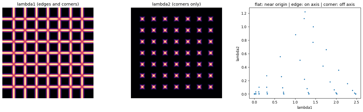
5. Eigenvalues classify the window

Diagonalizing the second moment matrix,

\[\begin{split} A = U \begin{bmatrix} \lambda_1 & 0 \\ 0 & \lambda_2 \end{bmatrix} U^\top, \end{split}\]

the eigenvalues measure intensity change along the two principal directions:

• \(\lambda_1, \lambda_2\) both small \(\rightarrow\) flat

• one large, one small \(\rightarrow\) edge

• both large \(\rightarrow\) corner

For a symmetric \(A = \begin{bmatrix} a & b \\ b & c \end{bmatrix}\) the eigenvalues have a closed form, which makes a per-pixel map cheap:

\[ \lambda_{1,2} = \frac{a + c}{2} \pm \sqrt{\left( \frac{a - c}{2} \right)^2 + b^2}. \]

chk = ndi.gaussian_filter(load_gray(data.checkerboard()), 1)
Ix, Iy = ndi.sobel(chk, axis=1), ndi.sobel(chk, axis=0)
a, b, c, lam1, lam2 = second_moment_eigs(Ix, Iy, sigma_w=2)

fig, ax = plt.subplots(1, 3, figsize=(15, 4.6))
show(ax[0], lam1, 'lambda1 (edges and corners)', cmap='magma')
show(ax[1], lam2, 'lambda2 (corners only)', cmap='magma')
sub = (slice(None, None, 3), slice(None, None, 3))   # subsample for the scatter
ax[2].scatter(lam1[sub].ravel(), lam2[sub].ravel(), s=3, alpha=0.2)
ax[2].set_xlabel('lambda1'); ax[2].set_ylabel('lambda2')
ax[2].set_title('flat: near origin | edge: on axis | corner: off axis')
plt.tight_layout(); plt.show()

6. The Harris corner detector

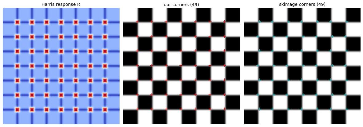
Computing eigenvalues at every pixel is avoidable. Harris (1988) uses a response built from the determinant and trace, which need only the entries of \(A\):

\[ M_c = \lambda_1 \lambda_2 - \kappa (\lambda_1 + \lambda_2)^2 = \det(A) - \kappa \, \mathrm{trace}^2(A), \qquad \kappa \in [0.04, 0.06]. \]

\(M_c\) is large and positive only when both eigenvalues are large. The full detector:

1. Compute gradients \(I_x, I_y\).

2. Form \(I_x^2, I_y^2, I_x I_y\) and smooth each with \(w\) to build \(A\) at every pixel.

3. Compute the response \(M_c = \det(A) - \kappa \, \mathrm{trace}^2(A)\).

4. Threshold \(M_c\).

5. Keep local maxima (non-maximum suppression).

def harris_response(im, sigma=1, sigma_w=2, kappa=0.05):
    g = ndi.gaussian_filter(im, sigma)
    Ix, Iy = ndi.sobel(g, axis=1), ndi.sobel(g, axis=0)
    a, b, c, _, _ = second_moment_eigs(Ix, Iy, sigma_w)
    det, trace = a*c - b*b, a + c
    return det - kappa * trace**2

def harris_corners(im, threshold_rel=0.05, **kw):
    R = harris_response(im, **kw)
    pts = peak_local_max(R, min_distance=8, threshold_rel=threshold_rel, exclude_border=8)
    return R, pts

chk = ndi.gaussian_filter(load_gray(data.checkerboard()), 1)
R, pts = harris_corners(chk)
ref = corner_peaks(corner_harris(chk), min_distance=8, threshold_rel=0.05, exclude_border=8)

fig, ax = plt.subplots(1, 3, figsize=(14, 4.8))
show(ax[0], R, 'Harris response R', cmap='coolwarm')
show(ax[1], chk, f'our corners ({len(pts)})');   ax[1].plot(pts[:, 1], pts[:, 0], 'r+', ms=9)
show(ax[2], chk, f'skimage corners ({len(ref)})'); ax[2].plot(ref[:, 1], ref[:, 0], 'c+', ms=9)
plt.tight_layout(); plt.show()

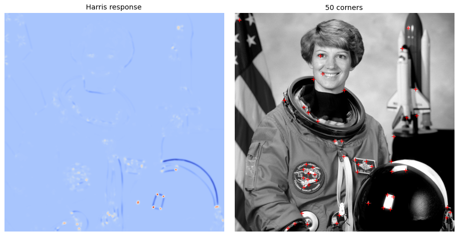
# the same detector on a natural image
astro = load_gray(data.astronaut())
Ra, pa = harris_corners(astro, threshold_rel=0.08)

fig, ax = plt.subplots(1, 2, figsize=(11, 5.5))
show(ax[0], Ra, 'Harris response', cmap='coolwarm')
show(ax[1], astro, f'{len(pa)} corners'); ax[1].plot(pa[:, 1], pa[:, 0], 'r+', ms=7)
plt.tight_layout(); plt.show()

.../site-packages/skimage/color/colorconv.py:984: RuntimeWarning: divide by zero encountered in matmul
  return rgb @ coeffs
.../site-packages/skimage/color/colorconv.py:984: RuntimeWarning: overflow encountered in matmul
  return rgb @ coeffs
.../site-packages/skimage/color/colorconv.py:984: RuntimeWarning: invalid value encountered in matmul
  return rgb @ coeffs

7. Cornerness measures and variants

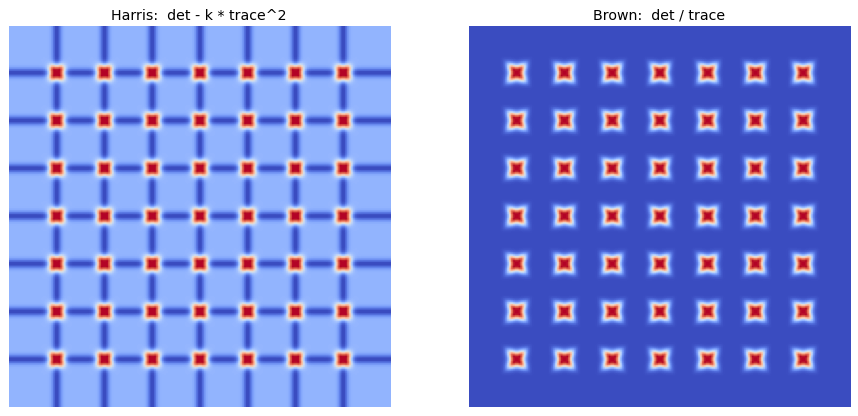
The same matrix \(A\) admits several cornerness scores, all functions of \(\lambda_0, \lambda_1\):

\[ \text{Harris-Stephens: } \det(A) - \alpha \, \mathrm{trace}^2(A) \qquad \text{Triggs: } \lambda_0 - \alpha \lambda_1 \qquad \text{Brown (harmonic mean): } \frac{\det(A)}{\mathrm{trace}(A)} = \frac{\lambda_0 \lambda_1}{\lambda_0 + \lambda_1}. \]

The harmonic mean is smoother near \(\lambda_0 \approx \lambda_1\) and needs no free parameter \(\kappa\). The two response maps below agree on corners but differ in how sharply they fall off.

def harmonic_mean_response(im, sigma=1, sigma_w=2, eps=1e-6):
    g = ndi.gaussian_filter(im, sigma)
    Ix, Iy = ndi.sobel(g, axis=1), ndi.sobel(g, axis=0)
    a, b, c, _, _ = second_moment_eigs(Ix, Iy, sigma_w)
    det, trace = a*c - b*b, a + c
    return det / (trace + eps)

chk = ndi.gaussian_filter(load_gray(data.checkerboard()), 1)
fig, ax = plt.subplots(1, 2, figsize=(11, 5))
show(ax[0], harris_response(chk),         'Harris:  det - k * trace^2', cmap='coolwarm')
show(ax[1], harmonic_mean_response(chk),  'Brown:  det / trace',        cmap='coolwarm')
plt.tight_layout(); plt.show()

8. Properties: rotation and scale

The response depends on \(A\), which behaves predictably under image transforms:

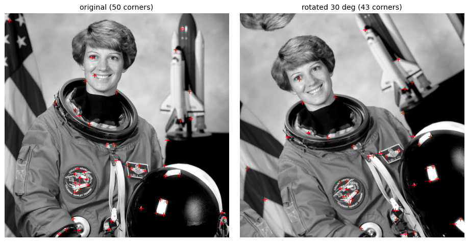
• Rotation: rotating the image rotates the eigenvectors of \(A\) but leaves the eigenvalues unchanged, so relative cornerness is preserved. Harris is rotation invariant.

• Photometric: only derivatives enter \(A\), so a brightness shift \(I \rightarrow I + b\) has no effect; a contrast scale \(I \rightarrow a I\) scales the response, so it is only partially invariant.

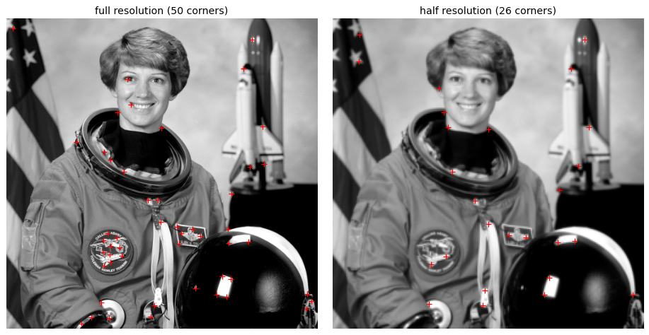
• Scale: a structure that is a corner under a small window becomes an edge under a large one. Harris is not scale invariant; the detected set changes with image scale.

# rotation: corners are found at corresponding points
astro = load_gray(data.astronaut())
_, p0 = harris_corners(astro, threshold_rel=0.08)
rot   = rotate(astro, 30, resize=False, mode='reflect')
_, p1 = harris_corners(rot, threshold_rel=0.08)

fig, ax = plt.subplots(1, 2, figsize=(11, 5.5))
show(ax[0], astro, f'original ({len(p0)} corners)'); ax[0].plot(p0[:, 1], p0[:, 0], 'r+', ms=6)
show(ax[1], rot,   f'rotated 30 deg ({len(p1)} corners)'); ax[1].plot(p1[:, 1], p1[:, 0], 'r+', ms=6)
plt.tight_layout(); plt.show()

# scale: the detected corner set is not preserved across resolutions
full = load_gray(data.astronaut())
half = ndi.gaussian_filter(full, 1)[::2, ::2]
_, pf = harris_corners(full, threshold_rel=0.08)
_, ph = harris_corners(half, threshold_rel=0.08)

fig, ax = plt.subplots(1, 2, figsize=(11, 5.5))
show(ax[0], full, f'full resolution ({len(pf)} corners)'); ax[0].plot(pf[:, 1], pf[:, 0], 'r+', ms=6)
show(ax[1], half, f'half resolution ({len(ph)} corners)'); ax[1].plot(ph[:, 1], ph[:, 0], 'r+', ms=6)
plt.tight_layout(); plt.show()

9. Explore and verify

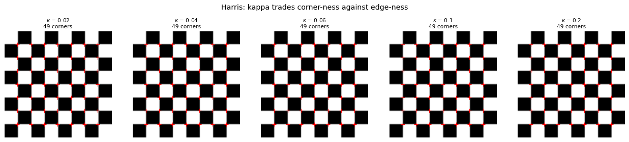
Two claims from this lecture are directly testable: that the Harris detector is invariant to rotation but not to scale, and that the eigenvalues of the second moment matrix separate flat, edge and corner windows. We test both, then sweep the detector’s knobs.

# Verify the invariance claims.
from skimage import transform
import scipy.ndimage as ndi

im = util.img_as_float(data.checkerboard())

# harris_corners returns (R, pts).
_, pts0  = harris_corners(im, threshold_rel=0.1)
_, pts90 = harris_corners(np.rot90(im), threshold_rel=0.1)
assert len(pts0) == len(pts90), f'rotation changed the corner count: {len(pts0)} vs {len(pts90)}'

big = transform.rescale(im, 2.0, anti_aliasing=True)
_, pts2x = harris_corners(big, threshold_rel=0.1)

# Eigenvalues classify the window. second_moment_eigs returns (a, b, c, lam1, lam2).
print('  window     lambda_max   lambda_min   expected')
for name, patch, expect in [('flat',   np.ones((40, 40)) * 0.5,               'both small'),
                            ('edge',   np.r_[np.zeros((40, 20)), np.ones((40, 20))].reshape(40, 40).T, 'one large'),
                            ('corner', np.pad(np.ones((20, 20)), ((20, 0), (20, 0))), 'both large')]:
    gx, gy = ndi.sobel(patch, axis=1), ndi.sobel(patch, axis=0)
    _, _, _, l1, l2 = second_moment_eigs(gx, gy, 2.0)
    print(f'  {name:8s} {l1.max():10.3f} {l2.max():12.3f}   {expect}')

print(f'\nrotation by 90 degrees: {len(pts0)} corners -> {len(pts90)} corners (invariant)')
print(f'scaling by 2x         : {len(pts0)} corners -> {len(pts2x)} corners (NOT invariant)')

  window     lambda_max   lambda_min   expected
  flat          0.000        0.000   both small
  edge          6.008        0.000   one large
  corner        6.008        2.935   both large

rotation by 90 degrees: 49 corners -> 49 corners (invariant)
scaling by 2x         : 49 corners -> 49 corners (NOT invariant)

# Static sweep: the sensitivity parameter kappa.
fig, ax = plt.subplots(1, 5, figsize=(15, 3.2))
for a, kap in zip(ax, [0.02, 0.04, 0.06, 0.10, 0.20]):
    _, pts = harris_corners(im, threshold_rel=0.1, kappa=kap)
    a.imshow(im, cmap='gray'); a.set_axis_off()
    if len(pts): a.plot(pts[:, 1], pts[:, 0], 'r+', ms=6)
    a.set_title(f'$\kappa$ = {kap}\n{len(pts)} corners', fontsize=9)
fig.suptitle('Harris: kappa trades corner-ness against edge-ness', y=1.02)
plt.tight_layout(); plt.show()

Now the same thing under your control. Drag the slider and watch what changes.

# Live: kappa and the detection threshold together.
from ipywidgets import interact, FloatSlider

def harris(kappa=0.04, threshold_rel=0.10):
    _, pts = harris_corners(im, threshold_rel=threshold_rel, kappa=kappa)
    fig, a = plt.subplots(figsize=(4.6, 4.6))
    a.imshow(im, cmap='gray'); a.set_axis_off()
    if len(pts): a.plot(pts[:, 1], pts[:, 0], 'r+', ms=7)
    a.set_title(f'$\kappa$={kappa:.3f}, threshold={threshold_rel:.2f}  ->  {len(pts)} corners')
    plt.show()

interact(harris,
         kappa=FloatSlider(min=0.01, max=0.25, step=0.01, value=0.04),
         threshold_rel=FloatSlider(min=0.02, max=0.50, step=0.02, value=0.10));

---

Key takeaways

Concept	Key takeaway
Second moment matrix	Eigen-analysis of a local \(2 \times 2\) matrix recurs for lines, blobs, and corners
Line segments	Orientation from the larger eigenvector; straightness from \(\lambda_2 / \lambda_1\)
Laplacian	\(\nabla^2 f\) has the \(3 \times 3\) kernel \([\,0,1,0;\,1,-4,1;\,0,1,0\,]\)
LoG	\(\nabla^2(f * g)\) smooths then takes the Laplacian; less noise sensitive
Blob detection	LoG is circularly symmetric; a blob of radius \(r\) peaks at \(\sigma \approx r / \sqrt{2}\) across scale
Autocorrelation	\(E_{AC}(\Delta u) \approx \Delta u^\top A \, \Delta u\) with \(A = w * [\,I_x^2, I_x I_y;\, I_x I_y, I_y^2\,]\)
Eigenvalues	Both small flat, one large edge, both large corner
Harris	\(M_c = \det(A) - \kappa \, \mathrm{trace}^2(A)\) avoids an explicit eigen-decomposition
Variants	Triggs \(\lambda_0 - \alpha \lambda_1\); Brown harmonic mean \(\det(A) / \mathrm{trace}(A)\)
Invariance	Rotation invariant, partially photometric invariant, not scale invariant

Reading: Szeliski, Computer Vision: Algorithms and Applications, Ch. 2; Forsyth and Ponce, Computer Vision: A Modern Approach, Ch. 5.

References: C. Harris and M. Stephens (1988); B. Triggs (2004); M. Brown, R. Szeliski, S. Winder (2005). Slide sources: K. Grauman, R. Urtasun, S. Seitz, N. Snavely, S. Lazebnik, D. Hoiem.

Exercises

1. Rotation yes, scale no. Rotate a patch and confirm the Harris response is stable; then rescale it and show the response is not. Explain what breaks, using the fixed window size.

2. Cornerness measures compared. Sweep Harris’s \(k\) and compare the detections against the Shi-Tomasi \(\min(\lambda_1, \lambda_2)\) measure. Where do the two disagree?

3. Verify the blob scale law. For synthetic disks of several radii, find the \(\sigma\) that maximises the scale-normalized LoG and check it against \(\sigma^\star \approx r/\sqrt{2}\).

4. Read the eigenvalues. For a flat patch, an edge and a corner, print \((\lambda_1, \lambda_2)\) and classify each by hand. Confirm your labels match the detector’s output.