
📺 Lecture video | 📄 Slides
Week 5, Lecture 4: Visualizing CNNs#
NPTEL Deep Learning for Computer Vision | Prof. Vineeth N Balasubramanian, IIT Hyderabad
Companion notebook for §5.4 Visualizing CNNs.
A trained CNN is not a black box we have to accept on faith. This lecture builds six practical tools for looking inside a pretrained ResNet-18 and asking what has it learned and what is it looking at.
What you will learn
Visualize the first-layer filters and see the Gabor-like edge and color detectors they learn.
Visualize intermediate activations (feature maps) using forward hooks.
Find the maximally activating images for a chosen neuron.
Run an occlusion experiment to build a class-saliency heatmap (Zeiler and Fergus, 2014).
Compute a fast gradient saliency map with a single backward pass.
Visualize the penultimate representation space with PCA and t-SNE.
Contents
Load the model and a sample image
Method 1: First-layer filters
Method 2: Visualize activations (feature maps)
Method 3: Maximally activating images
Method 4: Occlusion experiment (Zeiler and Fergus, 2014)
Method 5: Gradient saliency (a fast complement to occlusion)
Method 6: Representation space (last layer)
How to run
Self-contained. Every setup step runs inside the notebook; the only downloads are the pretrained ResNet-18 weights and a small CIFAR-10 subset.
Runs on CPU or GPU, locally or on Google Colab. All cells are tuned to finish in a few seconds.
Interactive. Several cells end in a widget: run the cell, then drag the slider or pick from the dropdown and watch the figure update.
Read the short “What to notice” prompt near each widget so you know what to look for.
Review#
The previous lecture reused a pretrained network on a new task, freezing and unfreezing layers to trade between feature extraction and full fine-tuning. That treats the network as a working black box. This lecture opens it up and asks what it has actually learned.
Setup#
# Setup: runs on CPU or GPU, on Colab or locally.
import sys, math, time
import numpy as np
import torch
import torch.nn as nn
import torch.nn.functional as F
import matplotlib.pyplot as plt

# ipywidgets is preinstalled on Colab; install only if missing.
try:
    import ipywidgets as widgets
    from ipywidgets import interact, interactive
except ImportError:
    import subprocess
    subprocess.run([sys.executable, "-m", "pip", "install", "-q", "ipywidgets"])
    import ipywidgets as widgets
    from ipywidgets import interact, interactive

torch.manual_seed(0)
np.random.seed(0)
device = torch.device('cuda' if torch.cuda.is_available() else 'cpu')
print('Using device:', device)

def count_params(module):
    # Total number of parameters in a module.
    return sum(p.numel() for p in module.parameters())

def count_trainable(module):
    return sum(p.numel() for p in module.parameters() if p.requires_grad)

plt.rcParams['figure.dpi'] = 110
plt.rcParams['font.size'] = 10
Using device: cpu
1. Load the model and a sample image#
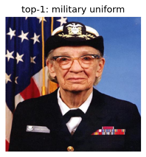
We use a pretrained ResNet-18 from torchvision (trained on ImageNet, 1000 classes). We read the human-readable class names straight from the weights metadata, so no label file needs downloading.
Our test image is grace_hopper.jpg, which ships with matplotlib. Before probing the network we
confirm it actually works by printing its top-5 predictions.
from torchvision.models import resnet18, ResNet18_Weights
from torchvision import transforms
import matplotlib.cbook as cbook
from PIL import Image

weights = ResNet18_Weights.DEFAULT
categories = weights.meta['categories']          # 1000 ImageNet class names, no download
model = resnet18(weights=weights).eval().to(device)
print('Model params:', f'{count_params(model):,}')
print('Number of classes:', len(categories))

# ImageNet preprocessing (matches how the model was trained).
preprocess = transforms.Compose([
    transforms.Resize(256), transforms.CenterCrop(224), transforms.ToTensor(),
    transforms.Normalize(mean=[0.485, 0.456, 0.406], std=[0.229, 0.224, 0.225]),
])
mean = torch.tensor([0.485, 0.456, 0.406]).view(1, 3, 1, 1)
std  = torch.tensor([0.229, 0.224, 0.225]).view(1, 3, 1, 1)

def load_sample_image(size=224):
    with cbook.get_sample_data('grace_hopper.jpg') as f:
        img = Image.open(f).convert('RGB').resize((size, size))
    return img

def denorm(x):
    # Undo ImageNet normalization for display; x is [3,H,W] or [B,3,H,W].
    x = x.detach().cpu()
    if x.dim() == 3:
        x = x.unsqueeze(0)
    x = (x * std + mean).clamp(0, 1)
    return x

sample_img = load_sample_image(224)
x_sample = preprocess(sample_img).unsqueeze(0).to(device)   # [1,3,224,224]

with torch.no_grad():
    probs = model(x_sample).softmax(dim=1)[0]
top5 = probs.topk(5)
print('\nTop-5 predictions for the sample image:')
for p, idx in zip(top5.values, top5.indices):
    print(f'  {p.item():5.3f}  {categories[idx]}')

fig, ax = plt.subplots(figsize=(3.2, 3.2))
ax.imshow(sample_img); ax.set_title(f'top-1: {categories[top5.indices[0]]}'); ax.axis('off')
plt.show()
Model params: 11,689,512
Number of classes: 1000

Top-5 predictions for the sample image:
  0.670  military uniform
  0.043  bow tie
  0.030  bearskin
  0.024  bulletproof vest
  0.023  academic gown
2. Method 1: First-layer filters#
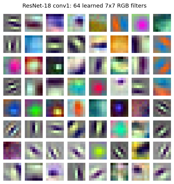
Why. The first convolution acts directly on RGB pixels, so its weights are directly interpretable as small image patches. Deeper kernels act on feature maps, not pixels, so their raw weights are not visually meaningful.
What to expect. The 64 filters of ResNet-18’s conv1 (shape 64 x 3 x 7 x 7) typically look
like Gabor-like oriented edge detectors and color blobs, the same primitives found in early
visual cortex and in almost every CNN regardless of architecture.
Each filter is normalized to [0, 1] independently before display.
W = model.conv1.weight.data.clone().cpu()      # [64, 3, 7, 7]
print('conv1 weight shape:', tuple(W.shape))

# Normalize every filter independently to [0,1] so its color pattern is visible.
Wn = torch.empty_like(W)
for i in range(W.shape[0]):
    f = W[i]
    Wn[i] = (f - f.min()) / (f.max() - f.min() + 1e-8)

fig, axes = plt.subplots(8, 8, figsize=(6.5, 6.5))
for i, ax in enumerate(axes.flat):
    ax.imshow(Wn[i].permute(1, 2, 0).numpy())
    ax.axis('off')
fig.suptitle('ResNet-18 conv1: 64 learned 7x7 RGB filters', y=0.93)
plt.show()
conv1 weight shape: (64, 3, 7, 7)
3. Method 2: Visualize activations (feature maps)#
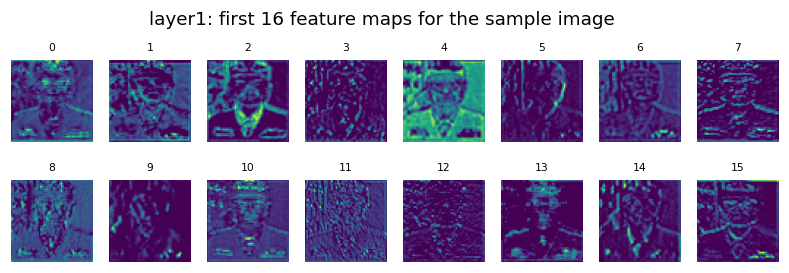
Why. A filter’s weights are static. Its activation (feature map) is what it actually outputs for a specific input. Feature maps show us where in the image each detector fires.
How. We attach forward hooks to named blocks layer1..layer4. A hook is a callback that
grabs a layer’s output during the forward pass without changing the model. We run the sample image
once and cache every activation.
What to notice. Early layers (layer1) respond to edges and textures and stay dense; deeper
layers (layer4) are more abstract and sparse, with fewer active locations. Spatial resolution
shrinks with depth (56, 28, 14, 7).
activations = {}
def make_hook(name):
    def hook(module, inp, out):
        activations[name] = out.detach().cpu()
    return hook

layer_names = ['layer1', 'layer2', 'layer3', 'layer4']
handles = [getattr(model, n).register_forward_hook(make_hook(n)) for n in layer_names]

with torch.no_grad():
    _ = model(x_sample)

for h in handles:      # remove hooks; activations dict is now populated
    h.remove()

for n in layer_names:
    print(f'{n:8s} activation shape: {tuple(activations[n].shape)}')
layer1   activation shape: (1, 64, 56, 56)
layer2   activation shape: (1, 128, 28, 28)
layer3   activation shape: (1, 256, 14, 14)
layer4   activation shape: (1, 512, 7, 7)
# WIDGET 1: pick a layer and a channel, see that single feature map.
def show_feature_map(layer='layer1', channel=0):
    act = activations[layer][0]                     # [C, H, W]
    c = min(channel, act.shape[0] - 1)
    fmap = act[c].numpy()
    fig, ax = plt.subplots(1, 2, figsize=(6.4, 3.2))
    ax[0].imshow(sample_img); ax[0].set_title('input'); ax[0].axis('off')
    im = ax[1].imshow(fmap, cmap='viridis')
    ax[1].set_title(f'{layer}  channel {c}/{act.shape[0]-1}  ({act.shape[1]}x{act.shape[2]})')
    ax[1].axis('off'); fig.colorbar(im, ax=ax[1], fraction=0.046)
    plt.show()

interact(show_feature_map,
         layer=widgets.Dropdown(options=layer_names, value='layer1', description='layer'),
         channel=widgets.IntSlider(min=0, max=511, step=1, value=0, description='channel'));
Try this: switch layer from layer1 to layer4 at a fixed channel. Notice the map gets
smaller and blockier and lights up in fewer places. Below is a static grid of the first 16 channels
of layer1 so you can compare detectors at a glance (many respond to oriented edges).
act1 = activations['layer1'][0]         # [64, 56, 56]
fig, axes = plt.subplots(2, 8, figsize=(9, 2.6))
for i, ax in enumerate(axes.flat):
    ax.imshow(act1[i].numpy(), cmap='viridis'); ax.axis('off'); ax.set_title(str(i), fontsize=7)
fig.suptitle('layer1: first 16 feature maps for the sample image', y=1.02)
plt.show()
A small image pool for the next experiments#
Methods 3 and 6 need many images. We load a CIFAR-10 subset (300 images), upsize to 96x96, and run one forward pass while two hooks capture:
the
layer2output (128 channels) for the maximally-activating-image search, andthe penultimate
avgpoolvector (512-dim) for the representation-space plot.
We compute this once and cache it so the widgets stay fast.
from torchvision import datasets
from torch.utils.data import Subset

cifar_classes = ['plane','car','bird','cat','deer','dog','frog','horse','ship','truck']
tf_disp = transforms.Compose([transforms.Resize(96), transforms.ToTensor()])   # 0..1, for display
pool_ds = datasets.CIFAR10(root='./data', train=False, download=True, transform=tf_disp)
N_POOL = 300
pool = Subset(pool_ds, range(N_POOL))

Xdisp = torch.stack([pool[i][0] for i in range(N_POOL)])          # [N,3,96,96] in 0..1
y_pool = torch.tensor([pool[i][1] for i in range(N_POOL)])
Xnorm = (Xdisp - mean) / std                                      # ImageNet-normalized

# Two hooks: layer2 mean activation per channel, and the 512-dim penultimate vector.
buf = {}
h2 = model.layer2.register_forward_hook(lambda m, i, o: buf.__setitem__('l2', o.detach().cpu()))
hp = model.avgpool.register_forward_hook(lambda m, i, o: buf.__setitem__('ap', o.detach().cpu()))

l2_means, feats = [], []
with torch.no_grad():
    for s in range(0, N_POOL, 50):
        _ = model(Xnorm[s:s+50].to(device))
        l2_means.append(buf['l2'].mean(dim=(2, 3)))               # [b,128]
        feats.append(buf['ap'].flatten(1))                        # [b,512]
h2.remove(); hp.remove()

l2_means = torch.cat(l2_means).numpy()      # [N,128]  mean activation per channel per image
feats = torch.cat(feats).numpy()            # [N,512]  penultimate features
print('layer2 mean-activation matrix:', l2_means.shape)
print('penultimate feature matrix:   ', feats.shape)
layer2 mean-activation matrix: (300, 128)
penultimate feature matrix:    (300, 512)
4. Method 3: Maximally activating images#
Why. To learn what a hidden neuron detects, find the images from a pool that make it fire the hardest. The common content across those images is (roughly) the pattern that neuron encodes, and the receptive-field patch that drives it is the concrete feature.
How. For a chosen layer2 channel we already stored its mean activation per image. We simply
sort the pool by that score and show the top-k images.
# WIDGET 2: pick a layer2 channel, see the images from the pool that activate it most.
def top_activating(channel=0, k=8):
    scores = l2_means[:, channel]
    order = np.argsort(-scores)[:k]
    fig, axes = plt.subplots(1, k, figsize=(1.5 * k, 1.8))
    for ax, idx in zip(axes, order):
        ax.imshow(Xdisp[idx].permute(1, 2, 0).numpy())
        ax.set_title(f'{cifar_classes[y_pool[idx]]}\n{scores[idx]:.2f}', fontsize=8)
        ax.axis('off')
    fig.suptitle(f'layer2 channel {channel}: top-{k} activating images (of {N_POOL})', y=1.15)
    plt.show()

interact(top_activating,
         channel=widgets.IntSlider(min=0, max=127, step=1, value=10, description='channel'),
         k=widgets.IntSlider(min=4, max=10, step=1, value=8, description='top-k'));
What to notice: as you scan channels, some neurons prefer a dominant color (blue sky or water), others prefer a shape or texture (round animal bodies, straight vehicle edges). The top images for one channel tend to share a visual theme, which is the neuron’s specialty.
5. Method 4: Occlusion experiment (Zeiler and Fergus, 2014)#
Why. Does the model use the object, or some background shortcut? Slide a small gray patch over the image; wherever hiding a region causes the biggest drop in the predicted-class probability is the region the model relies on. Plotting that probability over all patch positions gives a saliency heatmap.
How (efficiently). Naively this is one forward pass per patch position. Instead we stack every occluded variant into a single batch and run one forward pass. We use a modest 112x112 image and a coarse stride so it finishes in a moment.
img112 = load_sample_image(112)
# ToTensor then Normalize at 112x112 (reuse the last two preprocessing transforms).
x112 = preprocess.transforms[-1](preprocess.transforms[-2](img112)).unsqueeze(0).to(device)
with torch.no_grad():
    base_probs = model(x112).softmax(1)[0]
target = int(base_probs.argmax())
print(f'target class at 112x112: {categories[target]}  (p={base_probs[target]:.3f})')

def occlusion_heatmap(x, target, occ=24, stride=12):
    # Return an (rows x cols) grid of predicted-class prob with a gray patch at each position.
    _, C, H, Wd = x.shape
    tops = list(range(0, H, stride))
    lefts = list(range(0, Wd, stride))
    batch = []
    for t in tops:
        for l in lefts:
            v = x.clone()
            v[:, :, t:t+occ, l:l+occ] = 0.0        # 0 in normalized space is a neutral gray
            batch.append(v)
    batch = torch.cat(batch, 0)                    # [rows*cols, C, H, W], one big batch
    with torch.no_grad():
        p = model(batch).softmax(1)[:, target].cpu().numpy()
    return p.reshape(len(tops), len(lefts))

# WIDGET 3: occluder size and stride control the heatmap (coarser stride = fewer forward inputs).
def occlusion_demo(occ=24, stride=14):
    t0 = time.time()
    heat = occlusion_heatmap(x112, target, occ=occ, stride=stride)
    dt = time.time() - t0
    disp = denorm(x112)[0].permute(1, 2, 0).numpy()
    fig, ax = plt.subplots(1, 3, figsize=(9.5, 3.3))
    ax[0].imshow(disp); ax[0].set_title('image'); ax[0].axis('off')
    im = ax[1].imshow(heat, cmap='jet_r')          # dark red = big prob drop = important region
    ax[1].set_title(f'P({categories[target].split(",")[0]}) heatmap')
    ax[1].axis('off'); fig.colorbar(im, ax=ax[1], fraction=0.046)
    ax[2].imshow(disp)
    ax[2].imshow(heat, cmap='jet_r', alpha=0.55, extent=[0, 112, 112, 0], interpolation='bilinear')
    ax[2].set_title('overlay'); ax[2].axis('off')
    fig.suptitle(f'{heat.size} occluded variants in one batch, {dt:.2f}s', y=1.02)
    plt.show()

interact(occlusion_demo,
         occ=widgets.IntSlider(min=12, max=48, step=4, value=24, description='occluder'),
         stride=widgets.IntSlider(min=8, max=28, step=2, value=14, description='stride'));
target class at 112x112: bow tie (p=0.989)
Try this: shrink the stride for a finer, slower map and enlarge it for a coarse, fast map.
The darkest region (largest probability drop) marks the pixels the model most depends on for this
class. For grace_hopper the map concentrates on the uniform and face, not the background.
6. Method 5: Gradient saliency (a fast complement to occlusion)#
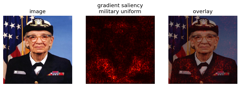
Why. Occlusion needs many forward passes. Gradient saliency answers a related question with a single backward pass: which input pixels, if nudged, would most change the class score?
How. Set requires_grad on the input, do one forward pass, backprop the top class score to the
pixels, and take the max absolute gradient across the three color channels:
$\(S(i,j) = \max_{c \in \{R,G,B\}} \left| \frac{\partial \, y_{\text{class}}}{\partial \, x_{c,i,j}} \right|.\)$
x_g = x_sample.clone().requires_grad_(True)
score = model(x_g)                                  # [1,1000]
cls = int(score.argmax())
model.zero_grad()
score[0, cls].backward()                            # one backward pass
sal = x_g.grad.detach().abs().amax(dim=1)[0].cpu().numpy()   # max over color channels -> [224,224]
sal = (sal - sal.min()) / (sal.max() - sal.min() + 1e-8)

fig, ax = plt.subplots(1, 3, figsize=(9.5, 3.3))
ax[0].imshow(sample_img); ax[0].set_title('image'); ax[0].axis('off')
ax[1].imshow(sal, cmap='hot'); ax[1].set_title(f'gradient saliency\n{categories[cls].split(",")[0]}')
ax[1].axis('off')
ax[2].imshow(sample_img); ax[2].imshow(sal, cmap='hot', alpha=0.5); ax[2].set_title('overlay')
ax[2].axis('off')
plt.show()
print('Bright pixels are the ones the class score is most sensitive to.')
Bright pixels are the ones the class score is most sensitive to.
7. Method 6: Representation space (last layer)#
Why. The penultimate 512-dim vector (just before the classifier) is the CNN’s compact code for an image. Two images with nearby codes are ones the network sees as semantically similar, not merely similar in raw pixels or color. Visualizing this space shows whether the model has organized images into meaningful clusters.
How. Project the 512-dim features of the pool to 2D two ways:
PCA: linear, fast, keeps the directions of largest variance.
t-SNE: nonlinear, slower, preserves local neighborhoods and tends to reveal tight clusters.
We color each point by its true CIFAR class.
from sklearn.decomposition import PCA
from sklearn.manifold import TSNE

pca_2d = PCA(n_components=2).fit_transform(feats)     # [N,2]
_tsne_cache = {}
def tsne_2d(perplexity):
    if perplexity not in _tsne_cache:
        _tsne_cache[perplexity] = TSNE(n_components=2, perplexity=perplexity,
                                       init='pca', learning_rate='auto',
                                       random_state=0).fit_transform(feats)
    return _tsne_cache[perplexity]

cmap10 = plt.get_cmap('tab10')
def scatter2d(ax, XY, title):
    yn = y_pool.numpy()
    for c in range(10):
        m = (yn == c)
        ax.scatter(XY[m, 0], XY[m, 1], s=14, color=cmap10(c), label=cifar_classes[c])
    ax.set_title(title); ax.set_xticks([]); ax.set_yticks([])

# WIDGET 4: switch between PCA and t-SNE (perplexity only affects t-SNE).
def repr_demo(method='PCA', perplexity=30):
    fig, ax = plt.subplots(figsize=(6.2, 5.2))
    if method == 'PCA':
        scatter2d(ax, pca_2d, 'PCA of 512-dim penultimate features')
    else:
        scatter2d(ax, tsne_2d(perplexity), f't-SNE (perplexity={perplexity})')
    ax.legend(markerscale=1.4, fontsize=7, loc='center left', bbox_to_anchor=(1.0, 0.5))
    plt.show()

interact(repr_demo,
         method=widgets.Dropdown(options=['PCA', 't-SNE'], value='PCA', description='method'),
         perplexity=widgets.IntSlider(min=5, max=50, step=5, value=30, description='perplexity'));
.../site-packages/sklearn/utils/extmath.py:335: RuntimeWarning: divide by zero encountered in matmul
  Q, _ = normalizer(A @ Q)
.../site-packages/sklearn/utils/extmath.py:335: RuntimeWarning: overflow encountered in matmul
  Q, _ = normalizer(A @ Q)
.../site-packages/sklearn/utils/extmath.py:335: RuntimeWarning: invalid value encountered in matmul
  Q, _ = normalizer(A @ Q)
.../site-packages/sklearn/utils/extmath.py:336: RuntimeWarning: divide by zero encountered in matmul
  Q, _ = normalizer(A.T @ Q)
.../site-packages/sklearn/utils/extmath.py:336: RuntimeWarning: overflow encountered in matmul
  Q, _ = normalizer(A.T @ Q)
.../site-packages/sklearn/utils/extmath.py:336: RuntimeWarning: invalid value encountered in matmul
  Q, _ = normalizer(A.T @ Q)
.../site-packages/sklearn/utils/extmath.py:340: RuntimeWarning: divide by zero encountered in matmul
  Q, _ = qr_normalizer(A @ Q)
.../site-packages/sklearn/utils/extmath.py:340: RuntimeWarning: overflow encountered in matmul
  Q, _ = qr_normalizer(A @ Q)
.../site-packages/sklearn/utils/extmath.py:340: RuntimeWarning: invalid value encountered in matmul
  Q, _ = qr_normalizer(A @ Q)
.../site-packages/sklearn/utils/extmath.py:533: RuntimeWarning: divide by zero encountered in matmul
  B = Q.T @ M
.../site-packages/sklearn/utils/extmath.py:533: RuntimeWarning: overflow encountered in matmul
  B = Q.T @ M
.../site-packages/sklearn/utils/extmath.py:533: RuntimeWarning: invalid value encountered in matmul
  B = Q.T @ M
.../site-packages/sklearn/utils/extmath.py:547: RuntimeWarning: divide by zero encountered in matmul
  U = Q @ Uhat
.../site-packages/sklearn/utils/extmath.py:547: RuntimeWarning: overflow encountered in matmul
  U = Q @ Uhat
.../site-packages/sklearn/utils/extmath.py:547: RuntimeWarning: invalid value encountered in matmul
  U = Q @ Uhat
What to notice: even though the model was never trained on CIFAR, its ImageNet features already separate the classes into groups (vehicles apart from animals, and so on). t-SNE usually shows tighter, rounder clusters than PCA; try a few perplexity values and watch the clusters tighten or merge.
Key takeaways: two families of methods#
Family |
Methods |
Idea |
|---|---|---|
Do not disturb the model |
first-layer filters, activations, maximally activating images, representation space |
read out what the fixed network already stores |
Perturb the input |
occlusion, gradient saliency |
change the input and watch the output move |
Filters show the primitive detectors learned in the first layer.
Activations show where those detectors fire for a specific image.
Maximally activating images reveal a neuron’s preferred pattern from data.
Representation space shows the global semantic geometry the model has built.
Occlusion and gradient saliency both localize the pixels responsible for a prediction, one by covering regions (many forward passes) and one by differentiation (a single backward pass).
Key takeaways#
First-layer filters are interpretable; deeper kernels are not (they act on feature maps, not pixels).
Forward hooks are the standard, non-invasive way to read any internal activation.
Maximally activating images turn an abstract neuron into a concrete visual concept.
Occlusion and gradient saliency are complementary: occlusion is model-agnostic but costly, gradients are cheap but noisier.
The penultimate features encode semantic similarity; PCA and t-SNE make that geometry visible.
Batching perturbations (as in the occlusion cell) is what keeps these experiments fast on a CPU.
Further reading#
Zeiler and Fergus, Visualizing and Understanding Convolutional Networks, ECCV 2014 (occlusion and deconvnet).
van der Maaten and Hinton, Visualizing Data using t-SNE, JMLR 2008.
Yosinski, Clune, Nguyen, Fuchs, Lipson, Understanding Neural Networks Through Deep Visualization, ICML DL Workshop 2014.
Stanford CS231n, Visualizing what ConvNets learn (course notes).
Exercises#
Occlusion patch size. Sweep the occluding patch size and describe the trade-off between a sharp map and a map that finds the whole object.
Saliency for the wrong class. Compute gradient saliency for the true class and for a class the image does not contain. What differs, and what does that tell you about how much to trust saliency?
What does this channel want? Pick a mid-level channel and find the images in a small set that activate it most. Name the pattern it appears to prefer.
Geometry of the representation. Project penultimate features to 2D and check whether classes separate. Compare against the same projection of raw pixels.