📺 Lecture video  |  📄 Slides

Watch on YouTube

Week 2, Lecture 6: Other Feature Spaces

NPTEL Deep Learning for Computer Vision | Prof. Vineeth N Balasubramanian, IIT Hyderabad

Companion notebook for §2.6 Other Feature Spaces.

What you will learn

• Describe shape with Shape Context.

• Detect stable regions with MSER.

• Build the HOG descriptor and its pyramidal variant PHOG.

• Encode texture with Local Binary Patterns (LBP).

• Compare these detectors and descriptors, and choose between them for a task.

Contents

1. Shape Context

2. Maximally Stable Extremal Regions (MSER)

3. Histogram of Oriented Gradients (HOG)

4. Pyramidal HOG (PHOG)

5. Local Binary Patterns (LBP)

6. Comparing feature detectors

How to run Runs on Colab or a local Jupyter, CPU only. Needs opencv-python alongside scikit-image and scipy; Colab ships all three. Run the setup cell first, then go top to bottom.

Review

Earlier lectures built detectors that fire at interesting locations: Harris corners, and blob detectors with a characteristic scale. A detector only says where; a descriptor says what, by turning a patch, region, or shape into a fixed-length vector that can be matched or fed to a classifier.

This lecture surveys the hand-crafted feature spaces that dominated recognition before deep learning:

• shape descriptors that compare object outlines (Shape Context),

• region descriptors from stable thresholded blobs (MSER),

• gradient descriptors from local orientation histograms (HOG, PHOG),

• texture descriptors from local intensity patterns (LBP).

Each one is a different answer to the same question: what is a good, invariant summary of local image content?

Setup

Everything runs offline on images bundled with scikit-image or generated synthetically. The load_gray and show helpers are shared across sections.

%matplotlib inline
import numpy as np
import matplotlib.pyplot as plt
from scipy import ndimage as ndi
from scipy.optimize import linear_sum_assignment
from skimage import data, util, color, feature
from skimage.measure import find_contours
import cv2

np.random.seed(0)
plt.rcParams['figure.figsize'] = (10, 4)
plt.rcParams['image.cmap']     = 'gray'
plt.rcParams['figure.dpi']     = 85

def load_gray(image):
    return color.rgb2gray(image) if image.ndim == 3 else util.img_as_float(image)

def show(ax, im, title='', cmap='gray'):
    ax.imshow(im, cmap=cmap); ax.set_title(title); ax.axis("off")

1. Shape Context

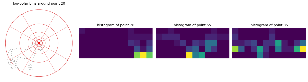
Shape Context describes a shape by how the rest of its outline is arranged around each boundary point. Sample \(N\) points on the contour. For a point \(p_i\), take the vectors to all other points and drop them into a log-polar histogram: bins are coarse in radius (log spacing) and uniform in angle, so nearby structure is measured finely and distant structure coarsely.

\[ h_i(k) = \#\{\, q \neq p_i : (q - p_i) \in \text{bin } k \,\}, \qquad k = 1, \dots, 60 . \]

Two properties follow from the construction:

• translation invariance, because only relative vectors are used,

• scale invariance, by normalizing the radii by their mean before binning.

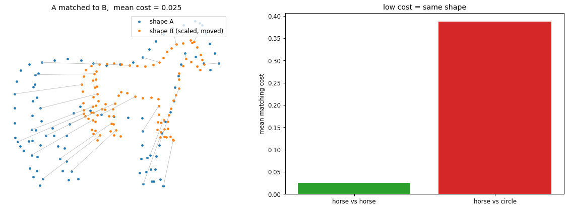
To compare a point \(i\) on one shape with a point \(j\) on another, the histograms are matched with a chi-square cost

\[ C_{ij} = \frac{1}{2} \sum_{k=1}^{K} \frac{\big[\, h_i(k) - h_j(k) \,\big]^2}{h_i(k) + h_j(k)} . \]

The best one-to-one correspondence minimizes the total cost, and a low total cost means the shapes match.

def sample_contour(mask, n_pts):
    c = max(find_contours(mask.astype(float), 0.5), key=len)   # longest boundary
    idx = np.linspace(0, len(c) - 1, n_pts).astype(int)
    return c[idx][:, ::-1]                                     # (row, col) -> (x, y)

def shape_context(pts, n_r=5, n_theta=12, r_min=0.125, r_max=2.0):
    d = pts[:, None, :] - pts[None, :, :]                      # vectors i -> j
    r = np.hypot(d[..., 0], d[..., 1])
    r = r / r[r > 0].mean()                                    # normalize radii -> scale invariant
    theta = np.arctan2(d[..., 1], d[..., 0]) % (2 * np.pi)
    r_edges = np.logspace(np.log10(r_min), np.log10(r_max), n_r + 1)
    r_bin = np.digitize(r, r_edges)                            # 0 (too near) .. n_r+1 (too far)
    t_bin = np.minimum((theta / (2 * np.pi) * n_theta).astype(int), n_theta - 1)
    N = len(pts); H = np.zeros((N, n_r, n_theta))
    for i in range(N):
        keep = (r_bin[i] >= 1) & (r_bin[i] <= n_r); keep[i] = False
        np.add.at(H[i], (r_bin[i][keep] - 1, t_bin[i][keep]), 1)
    H = H.reshape(N, -1)
    return H / (H.sum(1, keepdims=True) + 1e-8)                # per-point normalized histogram

pts = sample_contour(data.horse(), 100)
n_r, n_theta = 5, 12
H = shape_context(pts, n_r, n_theta)

d = pts[:, None, :] - pts[None, :, :]
mean_r = np.hypot(d[..., 0], d[..., 1])
mean_r = mean_r[mean_r > 0].mean()
edges_px = np.logspace(np.log10(0.125), np.log10(2.0), n_r + 1) * mean_r

ref = 20
fig, ax = plt.subplots(1, 4, figsize=(15, 4))
ax[0].plot(pts[:, 0], pts[:, 1], '.', ms=3, color='0.65')
ax[0].plot(*pts[ref], 'rs', ms=7)
for rad in edges_px:                                          # log-spaced radial bin edges
    ax[0].add_patch(plt.Circle(pts[ref], rad, fill=False, color='tab:red', lw=0.8))
for a in np.linspace(0, 2 * np.pi, n_theta, endpoint=False):  # angular bin edges
    ax[0].plot([pts[ref, 0], pts[ref, 0] + edges_px[-1] * np.cos(a)],
               [pts[ref, 1], pts[ref, 1] + edges_px[-1] * np.sin(a)], color='tab:red', lw=0.5)
ax[0].set_aspect('equal'); ax[0].invert_yaxis(); ax[0].axis('off')
ax[0].set_title(f'log-polar bins around point {ref}')
for k, i in enumerate([ref, 55, 85]):
    show(ax[k + 1], H[i].reshape(n_r, n_theta), f'histogram of point {i}', cmap='viridis')
plt.tight_layout(); plt.show()

.../site-packages/skimage/color/colorconv.py:984: RuntimeWarning: divide by zero encountered in matmul
  return rgb @ coeffs
.../site-packages/skimage/color/colorconv.py:984: RuntimeWarning: overflow encountered in matmul
  return rgb @ coeffs
.../site-packages/skimage/color/colorconv.py:984: RuntimeWarning: invalid value encountered in matmul
  return rgb @ coeffs

def sc_cost(HA, HB):                                          # chi-square between all point pairs
    a, b = HA[:, None, :], HB[None, :, :]
    return 0.5 * (((a - b) ** 2) / (a + b + 1e-8)).sum(-1)

def match(HA, HB):
    C = sc_cost(HA, HB)
    ri, ci = linear_sum_assignment(C)                         # optimal one-to-one correspondence
    return ci, C[ri, ci].mean()

A = sample_contour(data.horse(), 100)
B = A * 0.6 + [130, 40] + np.random.normal(0, 1.2, A.shape)   # same horse: scaled, moved, jittered

circ = np.zeros(data.horse().shape, bool)                     # a different shape for contrast
yy, xx = np.mgrid[:circ.shape[0], :circ.shape[1]]
circ[(xx - 200) ** 2 + (yy - 160) ** 2 < 90 ** 2] = True
C_pts = sample_contour(circ, 100)

HA, HB, HC = shape_context(A), shape_context(B), shape_context(C_pts)
corr, cost_same = match(HA, HB)
_, cost_diff = match(HA, HC)

fig, ax = plt.subplots(1, 2, figsize=(14, 5))
ax[0].plot(A[:, 0], A[:, 1], 'o', ms=3, color='tab:blue', label='shape A')
ax[0].plot(B[:, 0], B[:, 1], 'o', ms=3, color='tab:orange', label='shape B (scaled, moved)')
for i in range(0, 100, 4):
    ax[0].plot([A[i, 0], B[corr[i], 0]], [A[i, 1], B[corr[i], 1]], color='0.7', lw=0.6)
ax[0].invert_yaxis(); ax[0].set_aspect('equal'); ax[0].legend(loc='upper right')
ax[0].set_title(f'A matched to B,  mean cost = {cost_same:.3f}'); ax[0].axis('off')
ax[1].bar(['horse vs horse', 'horse vs circle'], [cost_same, cost_diff],
          color=['tab:green', 'tab:red'])
ax[1].set_ylabel('mean matching cost'); ax[1].set_title('low cost = same shape')
plt.tight_layout(); plt.show()

2. Maximally Stable Extremal Regions (MSER)

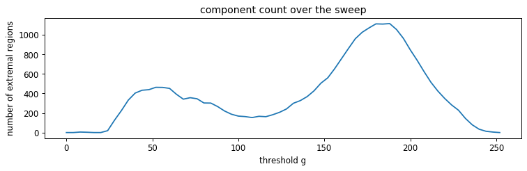
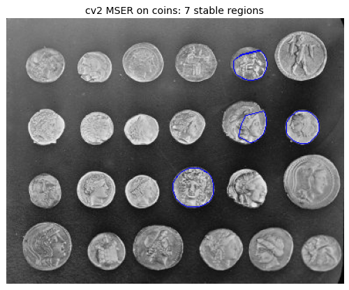
MSER detects blobs by watching how thresholded regions behave as the threshold moves. Sweep a gray level \(g\) from low to high and keep the connected components of the thresholded image. These are extremal regions: every pixel inside is brighter (or darker) than every pixel on the boundary. As \(g\) changes, regions are born, grow, and merge, which nests them in a tree.

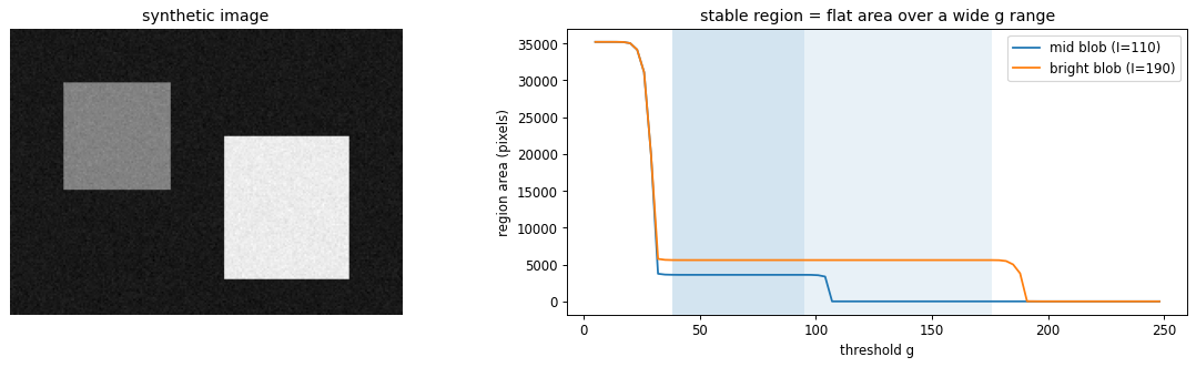
A region is stable if its area barely changes over a range of thresholds. With region areas \(|R^g|\) at level \(g\) and a small buffer \(\Delta\),

\[ \Psi(R^g) = \frac{|R^{g-\Delta}| - |R^{g+\Delta}|}{|R^g|} . \]

The regions where \(\Psi\) is a local minimum are the MSERs: they persist across many thresholds, which makes them repeatable under viewpoint and lighting changes. The descriptor is then the region itself (its shape, or a normalized patch).

img = util.img_as_ubyte(data.coins())

levels = np.linspace(40, 200, 6).astype(int)
fig, ax = plt.subplots(1, 7, figsize=(15, 3))
show(ax[0], img, 'input')
for k, g in enumerate(levels):
    show(ax[k + 1], img >= g, f'g = {g}')                     # bright extremal regions at level g
fig.suptitle('thresholding from dark to bright: extremal regions appear and merge')
plt.tight_layout(); plt.show()

gs = np.arange(0, 256, 4)
n_comp = [ndi.label(img >= g)[1] for g in gs]                 # connected components at each level
plt.figure(figsize=(9, 3))
plt.plot(gs, n_comp); plt.xlabel('threshold g'); plt.ylabel('number of extremal regions')
plt.title('component count over the sweep'); plt.tight_layout(); plt.show()

def region_area(im, seed, g):                                 # area of the region containing seed
    lab, _ = ndi.label(im >= g)
    lid = lab[seed]
    return (lab == lid).sum() if lid > 0 else 0

syn = np.full((160, 220), 30, np.float64)                     # two uniform blobs on a dark background
syn[30:90, 30:90]    = 110
syn[60:140, 120:190] = 190
syn = np.clip(syn + np.random.normal(0, 4, syn.shape), 0, 255)

seeds = {'mid blob (I=110)': (60, 60), 'bright blob (I=190)': (100, 155)}
gs = np.arange(5, 251, 3)

fig, ax = plt.subplots(1, 2, figsize=(14, 4))
show(ax[0], syn, 'synthetic image')
for name, seed in seeds.items():
    area = np.array([region_area(syn, seed, g) for g in gs], float)
    ax[1].plot(gs, area, label=name)
    D = 2                                                     # normalized area change over a buffer
    q = np.full_like(area, np.nan)
    q[D:-D] = np.abs(area[:-2 * D] - area[2 * D:]) / (area[D:-D] + 1e-8)
    stable = (q < 0.05) & (area > 50) & (area < 0.5 * syn.size)
    if stable.any():
        ax[1].axvspan(gs[stable][0], gs[stable][-1], alpha=0.10)   # shaded = stable plateau
ax[1].set_xlabel('threshold g'); ax[1].set_ylabel('region area (pixels)')
ax[1].set_title('stable region = flat area over a wide g range'); ax[1].legend()
plt.tight_layout(); plt.show()

gray = util.img_as_ubyte(data.coins())                        # what a library MSER returns
mser = cv2.MSER_create(delta=6, min_area=200, max_area=8000)
regions, _ = mser.detectRegions(gray)
canvas = cv2.cvtColor(gray, cv2.COLOR_GRAY2BGR)
for r in regions:
    cv2.polylines(canvas, [cv2.convexHull(r.reshape(-1, 1, 2))], True, (255, 0, 0), 1)
fig, ax = plt.subplots(figsize=(8, 5))
show(ax, canvas[..., ::-1], f'cv2 MSER on coins: {len(regions)} stable regions')
plt.tight_layout(); plt.show()

3. Histogram of Oriented Gradients (HOG)

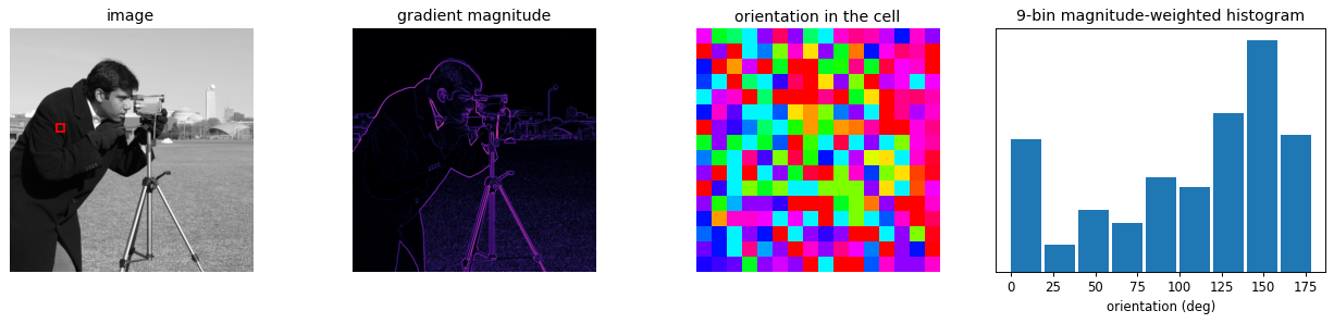
HOG summarizes local shape by the distribution of gradient orientations. The steps are:

1. Compute the gradient at every pixel, giving magnitude and orientation.

2. Split the image into small cells (say \(8 \times 8\) pixels).

3. In each cell build a histogram of orientations, where every pixel votes for its orientation bin weighted by its gradient magnitude.

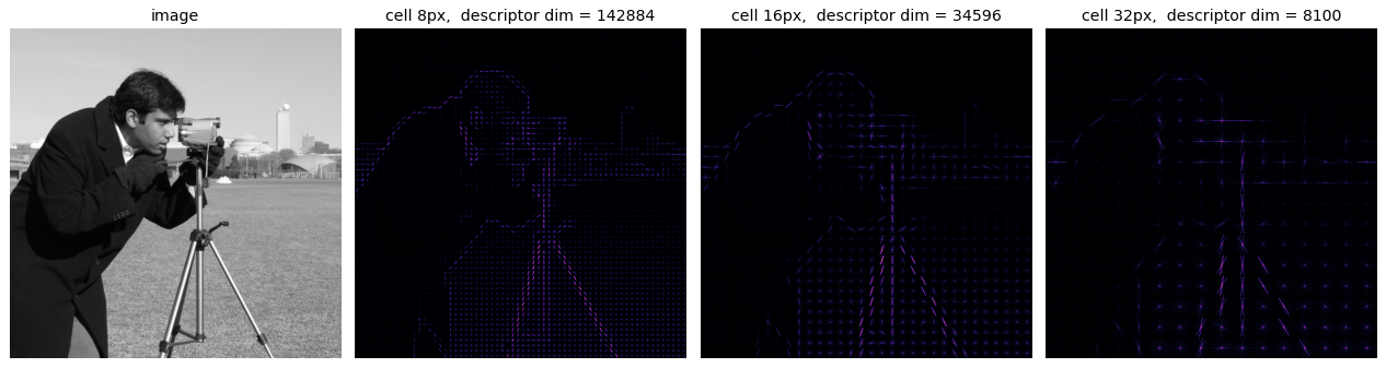
4. Group cells into overlapping blocks and normalize each block, which cancels local changes in contrast and illumination.

5. Concatenate all block histograms into the final descriptor.

Orientations are usually folded to \([0^\circ, 180^\circ)\) so that opposite gradient directions share a bin. The histogram keeps which orientations are present while discarding exactly where, which gives tolerance to small deformations. HOG was the standard for pedestrian detection before deep learning.

img = util.img_as_float(data.camera())
gy, gx = np.gradient(img)
mag = np.hypot(gx, gy)
ori = np.rad2deg(np.arctan2(gy, gx)) % 180                    # fold to [0, 180)

cy, cx, s = 200, 100, 16                                      # one 16x16 cell over a strong edge
cell_mag, cell_ori = mag[cy:cy + s, cx:cx + s], ori[cy:cy + s, cx:cx + s]
hist, edges = np.histogram(cell_ori, bins=9, range=(0, 180), weights=cell_mag)

fig, ax = plt.subplots(1, 4, figsize=(15, 3.6))
show(ax[0], img, 'image')
ax[0].add_patch(plt.Rectangle((cx, cy), s, s, ec='red', fc='none', lw=1.5))
show(ax[1], mag, 'gradient magnitude', cmap='magma')
show(ax[2], cell_ori, 'orientation in the cell', cmap='hsv')
ax[3].bar(edges[:-1], hist, width=18, align='edge', color='tab:blue')
ax[3].set_title('9-bin magnitude-weighted histogram')
ax[3].set_xlabel('orientation (deg)'); ax[3].set_yticks([])
plt.tight_layout(); plt.show()

from skimage.feature import hog

fig, ax = plt.subplots(1, 4, figsize=(15, 4))
show(ax[0], img, 'image')
for k, ppc in enumerate([(8, 8), (16, 16), (32, 32)]):
    feat, hog_img = hog(img, orientations=9, pixels_per_cell=ppc, cells_per_block=(2, 2),
                        visualize=True, feature_vector=True)
    show(ax[k + 1], hog_img, f'cell {ppc[0]}px,  descriptor dim = {feat.size}', cmap='magma')
plt.tight_layout(); plt.show()

4. Pyramidal HOG (PHOG)

HOG on one grid loses the coarse spatial layout of the shape. PHOG adds it back with a spatial pyramid. At level \(l\) the image is divided into \(2^l \times 2^l\) cells, an orientation histogram is taken over each cell, and the histograms from every level are concatenated:

\[ \text{PHOG} = \big[\; H^{(0)} \;\|\; H^{(1)} \;\|\; \dots \;\|\; H^{(L)} \;\big] . \]

Level \(0\) is a single global histogram; deeper levels record where the oriented edges sit. The concatenation captures the spatial arrangement of gradients better than a flat HOG, at the cost of a longer descriptor. With \(B\) orientation bins the length is \(B \sum_{l=0}^{L} 4^{l}\).

img = load_gray(data.astronaut())
edges = feature.canny(img, sigma=2)                           # PHOG histograms orientations on edges
gy, gx = np.gradient(img)
ori = np.rad2deg(np.arctan2(gy, gx)) % 180
mag = np.hypot(gx, gy) * edges                                # weight only edge pixels

def level_hist(ori, mag, l, bins=8):
    n = 2 ** l; Hh, Ww = ori.shape; feats = []
    for by in range(n):
        for bx in range(n):
            ys, xs = by * Hh // n, bx * Ww // n
            ye, xe = (by + 1) * Hh // n, (bx + 1) * Ww // n
            h, _ = np.histogram(ori[ys:ye, xs:xe], bins=bins, range=(0, 180),
                                weights=mag[ys:ye, xs:xe])
            feats.append(h)
    return np.concatenate(feats)

fig, ax = plt.subplots(2, 3, figsize=(14, 6))
for l in range(3):
    show(ax[0, l], edges, f'level l = {l}:  {2 ** l} x {2 ** l} grid')
    n = 2 ** l
    for g in range(1, n):                                     # draw the grid lines
        ax[0, l].axhline(g * img.shape[0] / n, color='lime', lw=0.8)
        ax[0, l].axvline(g * img.shape[1] / n, color='lime', lw=0.8)
    h = level_hist(ori, mag, l)
    ax[1, l].bar(range(len(h)), h, color='tab:green')
    ax[1, l].set_title(f'cell histograms concatenated ({len(h)} bins)'); ax[1, l].set_yticks([])
plt.tight_layout(); plt.show()

phog = np.concatenate([level_hist(ori, mag, l) for l in range(3)])
print('PHOG descriptor length (levels 0-2, 8 bins):', phog.size)

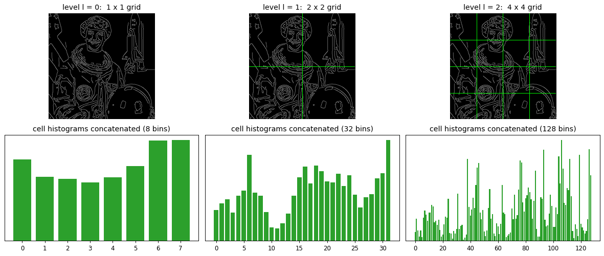
PHOG descriptor length (levels 0-2, 8 bins): 168

5. Local Binary Patterns (LBP)

LBP describes texture by comparing each pixel to its neighbors. For a pixel and its 8 neighbors, threshold each neighbor against the center: \(1\) if it is greater or equal, \(0\) otherwise. Reading the 8 bits in a fixed order gives a number in \([0, 255]\), the LBP code of that pixel.

\[\begin{split} \text{LBP}(c) = \sum_{p=0}^{P-1} s\big( g_p - g_c \big)\, 2^{p}, \qquad s(x) = \begin{cases} 1 & x \geq 0 \\ 0 & x < 0 \end{cases} \end{split}\]

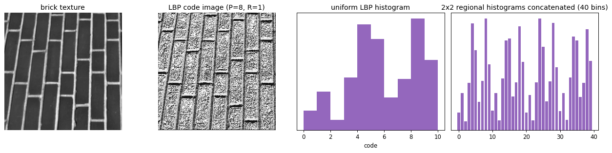
The code is a tiny signature of the local pattern (edge, corner, flat, spot). A texture is described by the histogram of codes over a region, and an image by concatenating the histograms of its cells. Two useful generalizations:

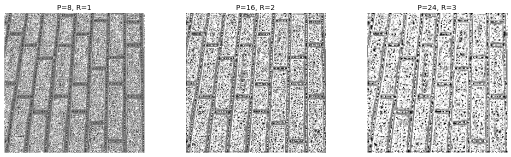
• a circle of \(P\) points at radius \(R\), with bilinear interpolation when a point falls between pixels, so different scales of texture can be captured,

• uniform patterns, which keep only codes with at most two bit transitions (the common edge and corner patterns) and pool the rest, shrinking the histogram.

patch = np.array([[116, 116, 128],
                  [254, 209, 155],
                  [255, 252, 252]])
c = patch[1, 1]
order = [(0, 0), (0, 1), (0, 2), (1, 2), (2, 2), (2, 1), (2, 0), (1, 0)]   # clockwise from top-left
bits = [1 if patch[i, j] >= c else 0 for i, j in order]
code = int(''.join(map(str, bits)), 2)
thr = (patch >= c).astype(int)

def grid_text(ax, values, center_label=None, title=''):
    ax.imshow(np.ones((3, 3)), cmap='gray', vmin=0, vmax=1)
    for i in range(3):
        for j in range(3):
            t = center_label if (center_label is not None and i == 1 and j == 1) else str(values[i, j])
            ax.text(j, i, t, ha='center', va='center', fontsize=13)
    ax.set_xticks(np.arange(-.5, 3, 1), minor=True)
    ax.set_yticks(np.arange(-.5, 3, 1), minor=True)
    ax.grid(which='minor', color='0.6', lw=1); ax.tick_params(length=0)
    ax.set_xticks([]); ax.set_yticks([]); ax.set_title(title)

fig, ax = plt.subplots(1, 3, figsize=(12, 3.6))
grid_text(ax[0], patch, title=f'3x3 patch  (center = {c})')
grid_text(ax[1], thr, center_label='c', title='neighbor >= center ?')
ax[2].axis('off')
ax[2].text(0.5, 0.62, 'bits, clockwise from top-left', ha='center', fontsize=12)
ax[2].text(0.5, 0.44, ''.join(map(str, bits)), ha='center', fontsize=22, family='monospace')
ax[2].text(0.5, 0.20, f'decimal code = {code}', ha='center', fontsize=15, color='tab:red')
plt.tight_layout(); plt.show()
print('binary', ''.join(map(str, bits)), '-> decimal', code, '  (slide: 00001111 = 15)')

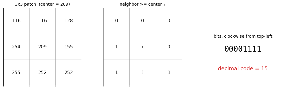
binary 00001111 -> decimal 15   (slide: 00001111 = 15)

from skimage.feature import local_binary_pattern

tex = util.img_as_ubyte(load_gray(data.brick()))[:256, :256]  # integer image avoids interp warnings
lbp_u = local_binary_pattern(tex, P=8, R=1, method='uniform')
lbp_d = local_binary_pattern(tex, P=8, R=1, method='default')

fig, ax = plt.subplots(1, 4, figsize=(15, 3.8))
show(ax[0], tex, 'brick texture')
show(ax[1], lbp_d, 'LBP code image (P=8, R=1)')
concat = []                                                   # regional histograms, then concatenate
for by in range(2):
    for bx in range(2):
        cell = lbp_u[by * 128:(by + 1) * 128, bx * 128:(bx + 1) * 128]
        h, _ = np.histogram(cell.ravel(), bins=10, range=(0, 10))
        concat.append(h)
concat = np.concatenate(concat)
ax[2].hist(lbp_u.ravel(), bins=10, range=(0, 10), color='tab:purple')
ax[2].set_title('uniform LBP histogram'); ax[2].set_xlabel('code'); ax[2].set_yticks([])
ax[3].bar(range(len(concat)), concat, color='tab:purple')
ax[3].set_title(f'2x2 regional histograms concatenated ({len(concat)} bins)'); ax[3].set_yticks([])
plt.tight_layout(); plt.show()

fig, ax = plt.subplots(1, 3, figsize=(13, 3.8))                # radius sets the scale of texture
for k, (P, R) in enumerate([(8, 1), (16, 2), (24, 3)]):
    show(ax[k], local_binary_pattern(tex, P, R, method='uniform'), f'P={P}, R={R}')
plt.tight_layout(); plt.show()

6. Comparing feature detectors

Different detectors respond to different structures (corners, blobs, regions) and offer different invariances. The survey of Tuytelaars and Mikolajczyk (2008) summarizes the trade-offs. A compact version:

Detector	Finds	Rotation inv.	Scale inv.	Affine inv.	Repeatability	Efficiency
Harris	corners	yes	no	no	high	high
Hessian	blobs	yes	no	no	med	med
Harris-Laplace	corners	yes	yes	no	high	med
DoG (SIFT)	blobs	yes	yes	no	med	med
Harris-Affine	corners	yes	yes	yes	high	med
Hessian-Affine	blobs	yes	yes	yes	high	med
MSER	regions	yes	yes	yes	high	high

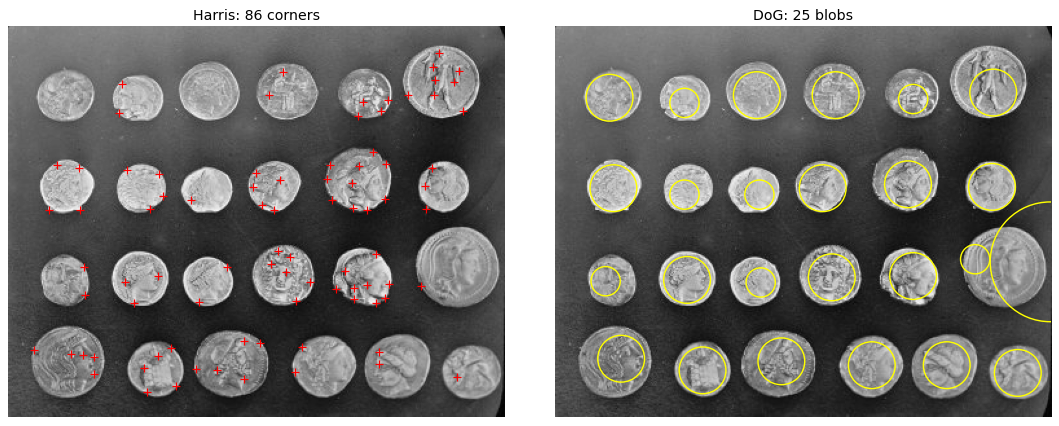
No single detector wins everywhere; the right choice depends on the transformation the images undergo and the compute budget. The demo below shows the most basic split: a corner detector (Harris) and a blob detector (DoG) firing on the same image.

from skimage.feature import corner_harris, corner_peaks, blob_dog

im = util.img_as_float(data.coins())
corners = corner_peaks(corner_harris(im), min_distance=6, threshold_rel=0.02)
blobs = blob_dog(im, min_sigma=8, max_sigma=35, threshold=0.05)  # small: peak DoG response here is ~0.09

fig, ax = plt.subplots(1, 2, figsize=(13, 5))
show(ax[0], im, f'Harris: {len(corners)} corners')
ax[0].plot(corners[:, 1], corners[:, 0], 'r+', ms=6)
show(ax[1], im, f'DoG: {len(blobs)} blobs')
for y, x, s in blobs:
    ax[1].add_patch(plt.Circle((x, y), s * np.sqrt(2), color='yellow', fill=False, lw=1.2))
plt.tight_layout(); plt.show()

7. Explore and verify

The descriptors in this lecture come with exact dimension arithmetic, and Shape Context comes with a matching cost that must vanish when a shape is matched against itself. Both are checkable.

# Verify the descriptor arithmetic.

# 1. HOG in the Dalal-Triggs setting: 64x128 window, 8x8 cells, 2x2 blocks, 9 bins.
win_w, win_h, cell_px, block, bins = 64, 128, 8, 2, 9
cells_x, cells_y = win_w // cell_px, win_h // cell_px               # 8 x 16
blocks_x, blocks_y = cells_x - block + 1, cells_y - block + 1       # 7 x 15
dim = blocks_x * blocks_y * block * block * bins
assert dim == 3780, f'HOG dimension came out as {dim}, expected 3780'
print(f'  HOG: {cells_x}x{cells_y} cells -> {blocks_x}x{blocks_y} blocks '
      f'-> {blocks_x}*{blocks_y}*{block * block}*{bins} = {dim} dimensions')

# 2. Shape Context: matching a shape to itself must cost essentially nothing.
#    sc_cost returns the full pairwise matrix; match() returns (assignment, mean cost).
mask = data.horse() == 0
P = sample_contour(mask, 80)
H = shape_context(P)
_, self_cost = match(H, H)
assert self_cost < 1e-6, f'self-match cost should be ~0, got {self_cost:.3e}'

Q = sample_contour(data.coins() > 120, 80)
_, other_cost = match(H, shape_context(Q))
assert other_cost > self_cost, 'a different shape did not cost more than a self-match'
print(f'  Shape Context: self-match cost = {self_cost:.2e}, different shape = {other_cost:.3f}')

  HOG: 8x16 cells -> 7x15 blocks -> 7*15*4*9 = 3780 dimensions
  Shape Context: self-match cost = 0.00e+00, different shape = 0.303

# Static sweep: LBP is a histogram of local binary codes; P sets its resolution.
from skimage.feature import local_binary_pattern

tex = load_gray(data.brick())
fig, ax = plt.subplots(1, 5, figsize=(15, 3.0))
for a, P in zip(ax, [4, 8, 12, 16, 24]):
    lbp = local_binary_pattern(tex, P=P, R=1.5, method='uniform')
    a.hist(lbp.ravel(), bins=P + 2, color='steelblue')
    a.set_title(f'P = {P} neighbours', fontsize=9); a.set_yticks([])
fig.suptitle('LBP: more neighbours, a finer texture code, a longer descriptor', y=1.04)
plt.tight_layout(); plt.show()

.../site-packages/skimage/feature/texture.py:360: UserWarning: Applying `local_binary_pattern` to floating-point images may give unexpected results when small numerical differences between adjacent pixels are present. It is recommended to use this function with images of integer dtype.
  warnings.warn(

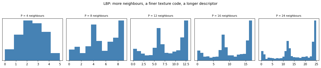
Now the same thing under your control. Drag the slider and watch what changes.

# Live: the LBP code map and its histogram together.
from ipywidgets import interact, IntSlider, FloatSlider

def lbp_view(P=8, Rr=1.5):
    lbp = local_binary_pattern(tex, P=P, R=Rr, method='uniform')
    fig, ax = plt.subplots(1, 2, figsize=(9.5, 3.8))
    ax[0].imshow(lbp, cmap='viridis'); ax[0].set_axis_off()
    ax[0].set_title(f'LBP codes, P={P}, R={Rr}')
    ax[1].hist(lbp.ravel(), bins=P + 2, color='steelblue'); ax[1].set_yticks([])
    ax[1].set_title(f'{P + 2}-bin uniform histogram')
    plt.tight_layout(); plt.show()

interact(lbp_view, P=IntSlider(min=4, max=24, step=4, value=8),
                   Rr=FloatSlider(min=1.0, max=4.0, step=0.5, value=1.5));

---

Key takeaways

Descriptor	Describes	Key idea	Invariances
Shape Context	shape outline	log-polar histogram of the other boundary points, matched by chi-square	translation, scale
MSER	regions	connected components stable across a range of thresholds	affine, illumination
HOG	local shape	magnitude-weighted histogram of gradient orientations per cell, block-normalized	small deformation, contrast
PHOG	global and local shape	HOG over a \(2^l \times 2^l\) pyramid, concatenated	adds coarse spatial layout
LBP	texture	histogram of per-pixel binary neighbor codes	grayscale-monotonic changes

Reading: Szeliski, Computer Vision: Algorithms and Applications, Ch. 4.1.1 and 4.1.2. Original papers: Belongie et al. (Shape Context, 2002), Matas et al. (MSER, 2004), Dalal and Triggs (HOG, 2005), Bosch et al. (PHOG, 2007), Ojala et al. (LBP, 1994).

To think about:

• All of these are hand-designed. What does a convolutional network learn in its early layers, and how does it compare to Gabor filters, HOG, and LBP?

• Shape Context needs a clean contour. What breaks it on a cluttered natural image?

• Why is MSER a good fit for detecting text in scenes?

Exercises

1. Check the HOG arithmetic. For the Dalal-Triggs setting (\(64\times128\) window, \(8\times8\) cells, \(2\times2\) blocks, 9 bins), derive the 3780-dimensional descriptor and confirm it against your implementation.

2. LBP invariances. Rotate a texture patch and compare plain LBP histograms against uniform rotation-invariant ones. Which claim of invariance actually holds?

3. Shape Context under transformation. Match a shape to a scaled and translated copy of itself, then to a different shape, and compare the chi-square costs.

4. MSER stability. Sweep the stability threshold and report how the number of detected regions responds. Which regions survive the widest range of thresholds?