
📺 Lecture video | 📄 Slides
Week 5, Lecture 2: More and Recent CNN Architectures#
NPTEL Deep Learning for Computer Vision | Prof. Vineeth N Balasubramanian, IIT Hyderabad
Companion notebook for §5.2 Recent CNN Architectures.
This lecture continues the story of convolutional network design past the original ResNet, walking through the modern ResNet family and the efficiency-focused blocks that power today’s vision models. We build each architecture’s signature block from scratch, verify its shapes and parameter cost, and explore its key hyperparameter with interactive sliders.
What you will learn
Build the modern ResNet-family and efficiency blocks from scratch and compare their compute cost.
Understand pre-activation ResNet (clean identity path) and WideResNet (width vs depth).
Understand ResNeXt cardinality via grouped convolutions, and DenseNet feature reuse via concatenation.
Understand MobileNet depthwise separable convolutions and quantify the FLOP savings.
Understand EfficientNet compound scaling, SENet channel attention, and the ConvNeXt modernizations.
Read parameter and FLOP counts to reason about the accuracy vs efficiency spectrum.
Contents
Recap: the residual block
Pre-activation ResNet (He et al., Identity Mappings, 2016)
Wide Residual Networks (Zagoruyko and Komodakis, 2016)
ResNeXt (Xie et al., 2017)
DenseNet (Huang et al., 2017)
MobileNet: depthwise separable convolution (Howard et al., 2017)
EfficientNet: compound scaling (Tan and Le, 2019)
SENet: Squeeze-and-Excitation (Hu et al., 2018)
ConvNeXt (Liu et al., 2022)
Cost comparison of the signature blocks
How to run
Self-contained: everything runs inside the notebook, no external downloads required (we only use small random tensors).
Runs on CPU or GPU, locally or on Google Colab. Every cell finishes in seconds; there is no training.
Interactive: several cells expose sliders and dropdowns. Run the cell, then drag the slider and watch the plot or numbers update.
Block-centric: for each architecture we build its key
nn.Module, check output shape and parameter count, and study one hyperparameter.
Review#
The previous lecture built the Inception module and the residual block, the two designs that made very deep networks trainable. This lecture follows what came after them: the ResNet variants, and the blocks designed for efficiency rather than raw accuracy.
Setup#
# Setup: runs on CPU or GPU, on Colab or locally.
import sys, math, time
import numpy as np
import torch
import torch.nn as nn
import torch.nn.functional as F
import matplotlib.pyplot as plt

# ipywidgets is preinstalled on Colab; install only if missing.
try:
    import ipywidgets as widgets
    from ipywidgets import interact, interactive
except ImportError:
    import subprocess
    subprocess.run([sys.executable, "-m", "pip", "install", "-q", "ipywidgets"])
    import ipywidgets as widgets
    from ipywidgets import interact, interactive

torch.manual_seed(0)
np.random.seed(0)
device = torch.device('cuda' if torch.cuda.is_available() else 'cpu')
print('Using device:', device)

def count_params(module):
    "Total number of parameters in a module."
    return sum(p.numel() for p in module.parameters())

def count_trainable(module):
    return sum(p.numel() for p in module.parameters() if p.requires_grad)

plt.rcParams['figure.dpi'] = 110
plt.rcParams['font.size'] = 10
Using device: cpu
1. Recap: the residual block#
Why it matters. The residual (skip) connection lets a block learn a residual \(F(x)\) that is added to the input: \(y = F(x) + x\). This keeps gradients flowing through very deep networks and made 100+ layer training practical.
The basic block (ResNet-18/34 style):
Two \(3\times3\) convolutions, each followed by BatchNorm and ReLU.
A skip connection adds the input to the output.
If the number of channels or the spatial size changes, the skip uses a \(1\times1\) conv to match shapes.
We build a small BasicBlock helper here and reuse the pattern throughout.
def conv3x3(cin, cout, stride=1):
    return nn.Conv2d(cin, cout, kernel_size=3, stride=stride, padding=1, bias=False)

class BasicBlock(nn.Module):
    "Standard post-activation residual block: conv-BN-ReLU x2 + skip."
    def __init__(self, cin, cout, stride=1):
        super().__init__()
        self.conv1 = conv3x3(cin, cout, stride)
        self.bn1   = nn.BatchNorm2d(cout)
        self.conv2 = conv3x3(cout, cout)
        self.bn2   = nn.BatchNorm2d(cout)
        # 1x1 projection on the skip if shape changes
        self.skip = nn.Sequential()
        if stride != 1 or cin != cout:
            self.skip = nn.Sequential(
                nn.Conv2d(cin, cout, kernel_size=1, stride=stride, bias=False),
                nn.BatchNorm2d(cout))
    def forward(self, x):
        out = F.relu(self.bn1(self.conv1(x)))
        out = self.bn2(self.conv2(out))
        out = out + self.skip(x)
        return F.relu(out)

blk = BasicBlock(64, 64)
x = torch.randn(1, 64, 32, 32)
y = blk(x)
print('input  :', tuple(x.shape))
print('output :', tuple(y.shape))
print('params :', count_params(blk))
input  : (1, 64, 32, 32)
output : (1, 64, 32, 32)
params : 73984
2. Pre-activation ResNet (He et al., Identity Mappings, 2016)#
Why it matters. In the original block the addition is followed by a ReLU, so the identity path is not truly clean: the signal that flows to the next block has already passed through a nonlinearity. Pre-activation moves BatchNorm and ReLU to before each convolution, leaving the skip path a pure identity. This improves gradient flow and lets even deeper nets (1000+ layers) train.
Ordering change:
Original:
conv -> BN -> ReLU(activation after conv, ReLU after the add).Pre-activation:
BN -> ReLU -> conv(activation before conv, nothing on the skip).
With pre-activation, \(y = x + F(x)\) where the \(+x\) path has no BN or ReLU on it, so gradients reach earlier layers unchanged.
class OriginalBlock(nn.Module):
    "conv -> BN -> ReLU (post-activation), ReLU after the add."
    def __init__(self, c):
        super().__init__()
        self.conv1, self.bn1 = conv3x3(c, c), nn.BatchNorm2d(c)
        self.conv2, self.bn2 = conv3x3(c, c), nn.BatchNorm2d(c)
    def forward(self, x):
        out = F.relu(self.bn1(self.conv1(x)))
        out = self.bn2(self.conv2(out))
        return F.relu(out + x)              # ReLU sits on the identity path

class PreActBlock(nn.Module):
    "BN -> ReLU -> conv (pre-activation); the skip stays a clean identity."
    def __init__(self, c):
        super().__init__()
        self.bn1, self.conv1 = nn.BatchNorm2d(c), conv3x3(c, c)
        self.bn2, self.conv2 = nn.BatchNorm2d(c), conv3x3(c, c)
    def forward(self, x):
        out = self.conv1(F.relu(self.bn1(x)))
        out = self.conv2(F.relu(self.bn2(out)))
        return out + x                      # nothing on the identity path

c = 64
xo = torch.randn(2, c, 16, 16)
ob, pb = OriginalBlock(c), PreActBlock(c)
print('Original   out:', tuple(ob(xo).shape), '| params:', count_params(ob))
print('PreAct     out:', tuple(pb(xo).shape), '| params:', count_params(pb))
print()
print('Original order : conv -> BN -> ReLU, then ReLU(out + x)')
print('PreAct   order : BN -> ReLU -> conv, then (out + x)  <- clean skip')
Original   out: (2, 64, 16, 16) | params: 73984
PreAct     out: (2, 64, 16, 16) | params: 73984

Original order : conv -> BN -> ReLU, then ReLU(out + x)
PreAct   order : BN -> ReLU -> conv, then (out + x)  <- clean skip
3. Wide Residual Networks (Zagoruyko and Komodakis, 2016)#
Why it matters. Instead of stacking ever more layers, WideResNet makes each block wider: multiply the number of filters by a width factor \(k\) (use \(F \cdot k\) filters). Key findings:
Width can beat depth: a shallower but wider net can match a much deeper thin one. A roughly 50-layer wide net can match a 152-layer ResNet.
Wider is more parallelizable on GPUs than deeper, because wide layers use larger, more efficient matrix multiplies.
Cost grows quadratically in \(k\) (both convs see \(k\times\) channels), so it is a knob to trade compute for accuracy.
Build a WideBlock with a width multiplier \(k\), then use a slider to watch the parameter count grow like \(k^2\).
class WideBlock(nn.Module):
    "Residual block whose base width F is multiplied by width factor k."
    def __init__(self, cin, F_base=16, k=1, stride=1):
        super().__init__()
        cout = F_base * k
        self.bn1, self.conv1 = nn.BatchNorm2d(cin), conv3x3(cin, cout, stride)
        self.bn2, self.conv2 = nn.BatchNorm2d(cout), conv3x3(cout, cout)
        self.skip = nn.Sequential()
        if stride != 1 or cin != cout:
            self.skip = nn.Conv2d(cin, cout, 1, stride=stride, bias=False)
    def forward(self, x):
        out = self.conv1(F.relu(self.bn1(x)))
        out = self.conv2(F.relu(self.bn2(out)))
        return out + self.skip(x)

for k in (1, 2, 4, 8):
    b = WideBlock(16, F_base=16, k=k)
    print(f'k={k:>2}  width={16*k:>3}  params={count_params(b):>8,}')
k= 1  width= 16  params=   4,672
k= 2  width= 32  params=  14,432
k= 4  width= 64  params=  47,264
k= 8  width=128  params= 168,224
Try this. Drag the \(k\) slider. Notice the parameter count scales roughly like \(k^2\): doubling the width roughly quadruples the parameters, because both the input and output channels of the inner conv grow with \(k\).
def wide_widget(F_base=16, k=1):
    fig, ax = plt.subplots(figsize=(6, 3.5))
    ks = np.arange(1, 13)
    params = [count_params(WideBlock(F_base, F_base=F_base, k=int(kk))) for kk in ks]
    ax.plot(ks, params, 'o-', color='steelblue')
    ax.scatter([k], [count_params(WideBlock(F_base, F_base=F_base, k=k))],
               color='crimson', zorder=5, s=80)
    ax.set_xlabel('width factor k'); ax.set_ylabel('parameters')
    ax.set_title(f'WideBlock params vs k  (F_base={F_base}, k={k}: '
                 f'{count_params(WideBlock(F_base, F_base=F_base, k=k)):,} params)')
    ax.grid(alpha=0.3)
    plt.show()

interact(wide_widget,
         F_base=widgets.IntSlider(min=8, max=64, step=8, value=16, description='F_base'),
         k=widgets.IntSlider(min=1, max=12, step=1, value=1, description='width k'));
4. ResNeXt (Xie et al., 2017)#
Why it matters. ResNeXt introduces a new dimension called cardinality: the number of parallel transformation pathways inside a block. It follows a split-transform-merge strategy (like Inception) but every pathway is identical and repeatable, so the block stays simple.
Cardinality = number of groups. Instead of one full convolution over all channels, split the channels into \(C\) groups and convolve each group independently. This is exactly a grouped convolution:
nn.Conv2d(..., groups=cardinality).A grouped conv with \(C\) groups costs about \(1/C\) of the FLOPs of the equivalent full-width conv, so you can increase cardinality instead of depth or width to gain accuracy at similar cost.
The block uses a \(1\times1\) reduce, a grouped \(3\times3\) transform, and a \(1\times1\) expand (a bottleneck).
Build a ResNeXtBlock, confirm the output shape is preserved, then use a slider to see how grouped conv is cheaper than a full-width conv.
class ResNeXtBlock(nn.Module):
    "Bottleneck block with a grouped 3x3 conv; groups = cardinality."
    def __init__(self, cin, cout, cardinality=32, width=4, stride=1):
        super().__init__()
        # bottleneck width scales with cardinality
        D = cardinality * width
        self.conv1 = nn.Conv2d(cin, D, 1, bias=False); self.bn1 = nn.BatchNorm2d(D)
        self.conv2 = nn.Conv2d(D, D, 3, stride=stride, padding=1,
                               groups=cardinality, bias=False); self.bn2 = nn.BatchNorm2d(D)
        self.conv3 = nn.Conv2d(D, cout, 1, bias=False); self.bn3 = nn.BatchNorm2d(cout)
        self.skip = nn.Sequential()
        if stride != 1 or cin != cout:
            self.skip = nn.Sequential(nn.Conv2d(cin, cout, 1, stride=stride, bias=False),
                                      nn.BatchNorm2d(cout))
    def forward(self, x):
        out = F.relu(self.bn1(self.conv1(x)))
        out = F.relu(self.bn2(self.conv2(out)))
        out = self.bn3(self.conv3(out))
        return F.relu(out + self.skip(x))

blk = ResNeXtBlock(256, 256, cardinality=32, width=4)
x = torch.randn(1, 256, 14, 14)
print('input :', tuple(x.shape), '-> output:', tuple(blk(x).shape))
print('params:', count_params(blk))
input : (1, 256, 14, 14) -> output: (1, 256, 14, 14)
params: 71168
Try this. Move the cardinality slider. We compare the grouped \(3\times3\) conv (the transform inside the block) against a single full-width \(3\times3\) conv over the same channels. Notice that raising cardinality shrinks the grouped conv cost, because each group only mixes \(1/C\) of the channels.
def resnext_widget(cardinality=32, width=4):
    D = cardinality * width
    grouped = nn.Conv2d(D, D, 3, padding=1, groups=cardinality, bias=False)
    full    = nn.Conv2d(D, D, 3, padding=1, groups=1, bias=False)
    pg, pf = count_params(grouped), count_params(full)

    fig, ax = plt.subplots(figsize=(6, 3.5))
    ax.bar(['grouped (C=%d)' % cardinality, 'full-width (C=1)'], [pg, pf],
           color=['seagreen', 'gray'])
    for i, v in enumerate([pg, pf]):
        ax.text(i, v, f'{v:,}', ha='center', va='bottom')
    ax.set_ylabel('params in the 3x3 conv')
    ax.set_title(f'D={D} channels  |  grouped is {pf/pg:.1f}x cheaper')
    plt.show()

interact(resnext_widget,
         cardinality=widgets.IntSlider(min=1, max=32, step=1, value=8, description='cardinality'),
         width=widgets.IntSlider(min=2, max=8, step=1, value=4, description='width'));
5. DenseNet (Huang et al., 2017)#
Why it matters. DenseNet takes feature reuse to the extreme: every layer receives the concatenation of ALL previous feature maps as its input, and passes its own output on to every later layer.
Each layer adds only a small number of channels, the growth rate \(k\). After \(L\) layers a block that started with \(C_{in}\) channels has \(C_{in} + L \cdot k\) channels.
Concatenation (not addition) means features are reused rather than summed, which strengthens gradient flow and makes the network parameter-efficient: each layer is thin, yet has access to all earlier features.
A
DenseLayerhere is BN -> ReLU -> \(3\times3\) conv producing \(k\) channels; aDenseBlockstacks \(L\) of them withtorch.cat.
Build them, verify the channel count grows as \(C_{in} + L\cdot k\), then explore \(k\) and \(L\) with sliders.
class DenseLayer(nn.Module):
    "BN -> ReLU -> 3x3 conv producing exactly k new channels."
    def __init__(self, cin, growth):
        super().__init__()
        self.bn, self.conv = nn.BatchNorm2d(cin), conv3x3(cin, growth)
    def forward(self, x):
        new = self.conv(F.relu(self.bn(x)))
        return torch.cat([x, new], dim=1)   # concatenate, do not add

class DenseBlock(nn.Module):
    def __init__(self, cin, growth=12, num_layers=6):
        super().__init__()
        layers, c = [], cin
        for _ in range(num_layers):
            layers.append(DenseLayer(c, growth)); c += growth
        self.block = nn.Sequential(*layers)
        self.out_channels = c
    def forward(self, x):
        return self.block(x)

Cin, k, L = 32, 12, 6
db = DenseBlock(Cin, growth=k, num_layers=L)
x = torch.randn(1, Cin, 28, 28)
y = db(x)
print(f'in channels : {Cin}')
print(f'out channels: {tuple(y.shape)[1]}  (formula C_in + L*k = {Cin} + {L}*{k} = {Cin + L*k})')
print(f'params      : {count_params(db):,}')
in channels : 32
out channels: 104  (formula C_in + L*k = 32 + 6*12 = 104)
params      : 40,920
Try this. Increase the growth rate \(k\) or the number of layers \(L\). The bar chart shows the channel width after each layer growing linearly, ending at \(C_{in} + L\cdot k\). Notice how a small \(k\) keeps each layer thin while the block still ends up wide.
def dense_widget(growth=12, num_layers=6, Cin=32):
    db = DenseBlock(Cin, growth=growth, num_layers=num_layers)
    channels = [Cin + i * growth for i in range(1, num_layers + 1)]
    fig, ax = plt.subplots(figsize=(6.5, 3.5))
    ax.bar(range(1, num_layers + 1), channels, color='mediumpurple')
    ax.set_xlabel('layer index'); ax.set_ylabel('channels after layer')
    ax.set_title(f'C_in={Cin}, k={growth}, L={num_layers}  ->  '
                 f'out={db.out_channels} ch, {count_params(db):,} params')
    plt.show()

interact(dense_widget,
         growth=widgets.IntSlider(min=4, max=48, step=4, value=12, description='growth k'),
         num_layers=widgets.IntSlider(min=1, max=16, step=1, value=6, description='layers L'),
         Cin=widgets.IntSlider(min=16, max=64, step=16, value=32, description='C_in'));
6. MobileNet: depthwise separable convolution (Howard et al., 2017)#
Why it matters. A standard \(k\times k\) conv mixes across space and across all channels at once, which is expensive. MobileNet factorizes it into two cheap steps:
Depthwise conv: one \(k\times k\) filter per input channel (
groups=C_in). It mixes only over space, not across channels.Pointwise conv: a \(1\times1\) conv that mixes across channels.
Cost reduction. For \(N\) output channels and kernel size \(k\), the depthwise separable conv costs a fraction
of a standard conv. For \(N=256, k=3\) that is about \(\tfrac{1}{256} + \tfrac{1}{9} \approx 0.115\), roughly an 8 to 9x reduction.
We build DepthwiseSeparableConv from scratch and verify the measured FLOP ratio matches \(1/N + 1/k^2\). We also introduce the width multiplier \(\alpha\) (scale channel counts) and resolution multiplier \(\rho\) (scale input resolution), both of which scale cost quadratically.
class DepthwiseSeparableConv(nn.Module):
    "Depthwise (per-channel kxk) followed by pointwise (1x1) convolution."
    def __init__(self, cin, cout, k=3, stride=1):
        super().__init__()
        self.depthwise = nn.Conv2d(cin, cin, k, stride=stride, padding=k // 2,
                                   groups=cin, bias=False)      # one filter per channel
        self.bn1 = nn.BatchNorm2d(cin)
        self.pointwise = nn.Conv2d(cin, cout, 1, bias=False)    # mix across channels
        self.bn2 = nn.BatchNorm2d(cout)
    def forward(self, x):
        x = F.relu(self.bn1(self.depthwise(x)))
        x = F.relu(self.bn2(self.pointwise(x)))
        return x

def conv_flops(cin, cout, k, H, W, groups=1):
    "Multiply-add count for a conv producing HxW output (per group accounting)."
    return (cin // groups) * cout * k * k * H * W

Cin, N, k, H, W = 128, 256, 3, 32, 32
# standard conv FLOPs
std = conv_flops(Cin, N, k, H, W)
# depthwise separable: depthwise (groups=Cin) + pointwise (1x1)
dw  = conv_flops(Cin, Cin, k, H, W, groups=Cin)
pw  = conv_flops(Cin, N, 1, H, W)
dsc = dw + pw

print(f'standard conv  FLOPs : {std:,}')
print(f'depthwise+point FLOPs: {dsc:,}  (dw {dw:,} + pw {pw:,})')
print(f'measured ratio dsc/std : {dsc/std:.4f}')
print(f'formula 1/N + 1/k^2    : {1/N + 1/k**2:.4f}')

# sanity check the module runs and preserves spatial size
m = DepthwiseSeparableConv(Cin, N, k=k)
xt = torch.randn(1, Cin, H, W)
print('module out shape:', tuple(m(xt).shape), '| params:', count_params(m))
standard conv  FLOPs : 301,989,888
depthwise+point FLOPs: 34,734,080  (dw 1,179,648 + pw 33,554,432)
measured ratio dsc/std : 0.1150
formula 1/N + 1/k^2    : 0.1150
module out shape: (1, 256, 32, 32) | params: 34688
Try this (answers the slide homework “by what fraction is computation reduced”). Set the kernel size \(k\), output channels \(N\), and spatial size, then compare standard vs depthwise separable FLOPs. The measured ratio should track the formula \(1/N + 1/k^2\) closely. Larger \(k\) and larger \(N\) both make the separable version relatively cheaper.
def dsc_widget(k=3, N=256, spatial=32, Cin=128):
    std = conv_flops(Cin, N, k, spatial, spatial)
    dsc = conv_flops(Cin, Cin, k, spatial, spatial, groups=Cin) + conv_flops(Cin, N, 1, spatial, spatial)
    ratio, formula = dsc / std, 1 / N + 1 / k**2

    fig, ax = plt.subplots(figsize=(6.5, 3.5))
    ax.bar(['standard', 'depthwise\nseparable'], [std, dsc], color=['gray', 'darkorange'])
    for i, v in enumerate([std, dsc]):
        ax.text(i, v, f'{v/1e6:.1f}M', ha='center', va='bottom')
    ax.set_ylabel('multiply-add FLOPs')
    ax.set_title(f'k={k}, N={N}, HxW={spatial}x{spatial}  |  '
                 f'ratio={ratio:.3f}  (1/N+1/k^2={formula:.3f}), '
                 f'{std/dsc:.1f}x cheaper')
    plt.show()

interact(dsc_widget,
         k=widgets.IntSlider(min=1, max=7, step=2, value=3, description='kernel k'),
         N=widgets.IntSlider(min=32, max=512, step=32, value=256, description='out N'),
         spatial=widgets.IntSlider(min=8, max=64, step=8, value=32, description='H=W'),
         Cin=widgets.IntSlider(min=32, max=256, step=32, value=128, description='in C'));
Width and resolution multipliers. MobileNet exposes two global knobs:
Width multiplier \(\alpha\): multiply every channel count by \(\alpha\). Cost scales like \(\alpha^2\) (both \(C_{in}\) and \(C_{out}\) shrink).
Resolution multiplier \(\rho\): multiply the input resolution by \(\rho\). Cost scales like \(\rho^2\) (fewer spatial positions \(H\times W\)).
The cell below shows both scalings on our example conv.
base = conv_flops(128, 256, 3, 32, 32)
print('base FLOPs:', f'{base:,}')
for alpha in (1.0, 0.75, 0.5, 0.25):
    c = conv_flops(int(128*alpha), int(256*alpha), 3, 32, 32)
    print(f'alpha={alpha:>4}: {c:>14,}  ({c/base:.3f}x, ~alpha^2={alpha**2:.3f})')
print()
for rho in (1.0, 0.857, 0.714, 0.571):   # e.g. 224,192,160,128 over 224
    s = int(round(32*rho))
    c = conv_flops(128, 256, 3, s, s)
    print(f'rho={rho:>5}: {c:>14,}  ({c/base:.3f}x, ~rho^2={rho**2:.3f})')
base FLOPs: 301,989,888
alpha= 1.0:    301,989,888  (1.000x, ~alpha^2=1.000)
alpha=0.75:    169,869,312  (0.562x, ~alpha^2=0.562)
alpha= 0.5:     75,497,472  (0.250x, ~alpha^2=0.250)
alpha=0.25:     18,874,368  (0.062x, ~alpha^2=0.062)

rho=  1.0:    301,989,888  (1.000x, ~rho^2=1.000)
rho=0.857:    214,990,848  (0.712x, ~rho^2=0.734)
rho=0.714:    156,008,448  (0.517x, ~rho^2=0.510)
rho=0.571:     95,551,488  (0.316x, ~rho^2=0.326)
7. EfficientNet: compound scaling (Tan and Le, 2019)#
Why it matters. Earlier nets scaled just one dimension (deeper, or wider, or higher resolution). EfficientNet scales all three together with a single compound coefficient \(\phi\):
subject to the constraint
Why that constraint? FLOPs grow linearly with depth but quadratically with width and resolution, so total FLOPs scale like \(\alpha \cdot \beta^2 \cdot \gamma^2\) raised to \(\phi\). Setting the product near \(2\) means each unit of \(\phi\) roughly doubles the FLOPs, so total cost grows as \(\approx 2^{\phi}\). The defaults from the paper are \(\alpha=1.2, \beta=1.1, \gamma=1.15\).
The widget below (answering the other slide homework) plots the FLOPs factor against \(\phi\) and shows it tracks \(2^{\phi}\).
def efficientnet_scaling(phi, alpha=1.2, beta=1.1, gamma=1.15):
    d = alpha ** phi           # depth multiplier
    w = beta  ** phi           # width multiplier
    r = gamma ** phi           # resolution multiplier
    flops_factor = d * (w ** 2) * (r ** 2)   # linear in depth, quadratic in width & res
    return d, w, r, flops_factor

for phi in range(0, 6):
    d, w, r, f = efficientnet_scaling(phi)
    print(f'phi={phi}: depth x{d:.2f}, width x{w:.2f}, res x{r:.2f}, '
          f'FLOPs x{f:.2f}  (2^phi = {2**phi})')
phi=0: depth x1.00, width x1.00, res x1.00, FLOPs x1.00  (2^phi = 1)
phi=1: depth x1.20, width x1.10, res x1.15, FLOPs x1.92  (2^phi = 2)
phi=2: depth x1.44, width x1.21, res x1.32, FLOPs x3.69  (2^phi = 4)
phi=3: depth x1.73, width x1.33, res x1.52, FLOPs x7.08  (2^phi = 8)
phi=4: depth x2.07, width x1.46, res x1.75, FLOPs x13.60  (2^phi = 16)
phi=5: depth x2.49, width x1.61, res x2.01, FLOPs x26.11  (2^phi = 32)
Try this. Drag \(\phi\) and optionally change \(\alpha, \beta, \gamma\). The red curve is the actual FLOPs factor \(\alpha^{\phi}\beta^{2\phi}\gamma^{2\phi}\); the dashed line is \(2^{\phi}\). With the default coefficients (whose product \(\alpha\beta^2\gamma^2 \approx 2\)) the two curves nearly coincide.
def compound_widget(phi=1.0, alpha=1.2, beta=1.1, gamma=1.15):
    d, w, r, f = efficientnet_scaling(phi, alpha, beta, gamma)
    phis = np.linspace(0, 6, 60)
    factors = [efficientnet_scaling(p, alpha, beta, gamma)[3] for p in phis]

    fig, ax = plt.subplots(figsize=(6.5, 4))
    ax.plot(phis, factors, color='crimson', label=r'$\alpha^\phi\beta^{2\phi}\gamma^{2\phi}$ (actual)')
    ax.plot(phis, 2**phis, '--', color='navy', label=r'$2^\phi$ (target)')
    ax.scatter([phi], [f], color='crimson', s=80, zorder=5)
    ax.set_xlabel(r'compound coefficient $\phi$'); ax.set_ylabel('FLOPs factor')
    ax.set_title(f'phi={phi:.1f}: depth x{d:.2f}, width x{w:.2f}, res x{r:.2f}, '
                 f'FLOPs x{f:.2f}\nproduct a*b^2*g^2 = {alpha*beta**2*gamma**2:.2f}')
    ax.legend(); ax.grid(alpha=0.3)
    plt.show()

interact(compound_widget,
         phi=widgets.FloatSlider(min=0, max=6, step=0.25, value=1.0, description='phi'),
         alpha=widgets.FloatSlider(min=1.0, max=1.6, step=0.05, value=1.2, description='alpha'),
         beta=widgets.FloatSlider(min=1.0, max=1.4, step=0.05, value=1.1, description='beta'),
         gamma=widgets.FloatSlider(min=1.0, max=1.4, step=0.05, value=1.15, description='gamma'));
8. SENet: Squeeze-and-Excitation (Hu et al., 2018)#
Why it matters. Not all channels are equally useful for a given input. SE blocks add cheap channel attention that learns to reweight channels per input.
Squeeze: global average pool each channel to a single number, giving a per-channel descriptor of length \(C\).
Excitation: a tiny bottleneck MLP, FC (reduce by ratio \(r\)) -> ReLU -> FC (restore to \(C\)) -> Sigmoid, producing a gate in \((0,1)\) for each channel.
Scale: multiply each channel of the feature map by its gate.
It is a plug-in module with very few parameters (set by the reduction ratio \(r\)) that recalibrates channel importance. Build SEBlock from scratch, apply it to a random feature map, and inspect the learned per-channel scales.
class SEBlock(nn.Module):
    "Squeeze-and-Excitation channel attention."
    def __init__(self, channels, reduction=16):
        super().__init__()
        hidden = max(1, channels // reduction)
        self.fc1 = nn.Linear(channels, hidden)
        self.fc2 = nn.Linear(hidden, channels)
    def forward(self, x):
        b, c, _, _ = x.shape
        s = x.mean(dim=(2, 3))              # squeeze: global average pool -> (b, c)
        s = F.relu(self.fc1(s))
        s = torch.sigmoid(self.fc2(s))      # excitation: gates in (0,1)
        return x * s.view(b, c, 1, 1), s    # scale each channel by its gate

C = 64
se = SEBlock(C, reduction=16)
x = torch.randn(1, C, 16, 16)
y, gates = se(x)
print('input :', tuple(x.shape), '-> output:', tuple(y.shape))
print('SE params:', count_params(se), '| gate range: '
      f'[{gates.min():.3f}, {gates.max():.3f}]')
input : (1, 64, 16, 16) -> output: (1, 64, 16, 16)
SE params: 580 | gate range: [0.381, 0.624]
Try this. Change the reduction ratio \(r\). A larger \(r\) means a tighter bottleneck and fewer parameters. The bar chart shows the per-channel attention gates the (untrained) block produces for a random input; after training these would emphasize the informative channels.
def se_widget(reduction=16, channels=64):
    torch.manual_seed(0)
    se = SEBlock(channels, reduction=reduction)
    x = torch.randn(1, channels, 16, 16)
    _, gates = se(x)
    g = gates.detach().numpy().ravel()

    fig, ax = plt.subplots(figsize=(7, 3.5))
    ax.bar(range(channels), g, color='teal')
    ax.axhline(0.5, color='gray', ls='--', lw=0.8)
    ax.set_xlabel('channel index'); ax.set_ylabel('attention gate (0,1)')
    ax.set_title(f'reduction r={reduction}: hidden={max(1, channels//reduction)}, '
                 f'SE params={count_params(se):,}')
    plt.show()

interact(se_widget,
         reduction=widgets.IntSlider(min=1, max=32, step=1, value=16, description='reduction r'),
         channels=widgets.IntSlider(min=16, max=128, step=16, value=64, description='channels'));
9. ConvNeXt (Liu et al., 2022)#
Why it matters. ConvNeXt asks: how far can a pure ConvNet go if we borrow the design choices that made Vision Transformers strong? The answer is a modernized ResNet that matches transformers. Key changes:
Patchify stem: a \(4\times4\), stride-4 conv that splits the image into non-overlapping patches (like a ViT tokenizer).
Depthwise conv with a large \(7\times7\) kernel: a big receptive field per channel, cheaply.
Inverted bottleneck: \(1\times1\) expand to a wider hidden dim, then \(1\times1\) reduce back.
Fewer activations and norms, GELU instead of ReLU, LayerNorm instead of BatchNorm.
Separate downsampling layers between stages.
Build a ConvNeXtBlock (depthwise \(7\times7\) -> LayerNorm -> \(1\times1\) expand -> GELU -> \(1\times1\) reduce -> residual add) and forward a random tensor.
class LayerNorm2d(nn.Module):
    "LayerNorm over the channel dim for (B, C, H, W) tensors."
    def __init__(self, c, eps=1e-6):
        super().__init__()
        self.weight = nn.Parameter(torch.ones(c))
        self.bias   = nn.Parameter(torch.zeros(c))
        self.eps = eps
    def forward(self, x):
        u = x.mean(1, keepdim=True)
        s = (x - u).pow(2).mean(1, keepdim=True)
        x = (x - u) / torch.sqrt(s + self.eps)
        return self.weight[None, :, None, None] * x + self.bias[None, :, None, None]

class ConvNeXtBlock(nn.Module):
    "Depthwise 7x7 -> LN -> 1x1 expand -> GELU -> 1x1 reduce, + residual."
    def __init__(self, dim, expansion=4):
        super().__init__()
        self.dwconv = nn.Conv2d(dim, dim, 7, padding=3, groups=dim)   # large-kernel depthwise
        self.norm   = LayerNorm2d(dim)
        self.pw1    = nn.Conv2d(dim, expansion * dim, 1)              # expand
        self.act    = nn.GELU()
        self.pw2    = nn.Conv2d(expansion * dim, dim, 1)             # reduce
    def forward(self, x):
        y = self.dwconv(x)
        y = self.norm(y)
        y = self.pw2(self.act(self.pw1(y)))
        return x + y                                                  # residual

dim = 96
blk = ConvNeXtBlock(dim, expansion=4)
x = torch.randn(1, dim, 28, 28)
print('input :', tuple(x.shape), '-> output:', tuple(blk(x).shape))
print('params:', count_params(blk), '| expansion=4')
input : (1, 96, 28, 28) -> output: (1, 96, 28, 28)
params: 79200 | expansion=4
Try this. The plot compares GELU (ConvNeXt) with ReLU. GELU is a smooth gate that lets small negative values through slightly, unlike ReLU’s hard cutoff at zero. The slider also lets you change the inverted-bottleneck expansion ratio and see its effect on the block’s parameter count.
def convnext_widget(expansion=4, dim=96):
    blk = ConvNeXtBlock(dim, expansion=expansion)
    z = torch.linspace(-4, 4, 200)
    gelu = F.gelu(z).numpy()
    relu = F.relu(z).numpy()

    fig, ax = plt.subplots(figsize=(6.5, 3.8))
    ax.plot(z.numpy(), gelu, color='crimson', label='GELU (ConvNeXt)')
    ax.plot(z.numpy(), relu, '--', color='navy', label='ReLU')
    ax.axhline(0, color='gray', lw=0.6); ax.axvline(0, color='gray', lw=0.6)
    ax.set_xlabel('input'); ax.set_ylabel('activation')
    ax.set_title(f'GELU vs ReLU  |  ConvNeXtBlock(dim={dim}, expansion={expansion}): '
                 f'{count_params(blk):,} params')
    ax.legend(); ax.grid(alpha=0.3)
    plt.show()

interact(convnext_widget,
         expansion=widgets.IntSlider(min=1, max=8, step=1, value=4, description='expansion'),
         dim=widgets.IntSlider(min=32, max=192, step=32, value=96, description='dim'));
10. Cost comparison of the signature blocks#
To feel the efficiency spectrum, we build one block per architecture at the same input and output channels and compare parameter counts. Depthwise separable and grouped blocks sit at the cheap end; wide and dense-heavy blocks sit at the expensive end. (Exact numbers depend on the internal width choices, but the ordering is the lesson.)
C = 128
blocks = {
    'BasicBlock':        BasicBlock(C, C),
    'PreAct':            PreActBlock(C),
    'Wide (k=2)':        WideBlock(C, F_base=C, k=2),
    'ResNeXt (C=32)':    ResNeXtBlock(C, C, cardinality=32, width=4),
    'DenseBlock (L=6)':  DenseBlock(C, growth=16, num_layers=6),
    'DepthwiseSep':      DepthwiseSeparableConv(C, C, k=3),
    'SEBlock (r=16)':    SEBlock(C, reduction=16),
    'ConvNeXt':          ConvNeXtBlock(C, expansion=4),
}
names  = list(blocks.keys())
params = [count_params(b) for b in blocks.values()]

fig, ax = plt.subplots(figsize=(9, 4))
bars = ax.bar(names, params, color='slateblue')
for b, p in zip(bars, params):
    ax.text(b.get_x() + b.get_width()/2, p, f'{p/1e3:.0f}k', ha='center', va='bottom', fontsize=8)
ax.set_ylabel('parameters'); ax.set_title(f'Signature block params at C_in=C_out={C}')
plt.xticks(rotation=30, ha='right'); plt.tight_layout()
plt.show()

for n, p in sorted(zip(names, params), key=lambda t: t[1]):
    print(f'{n:<20} {p:>10,} params')
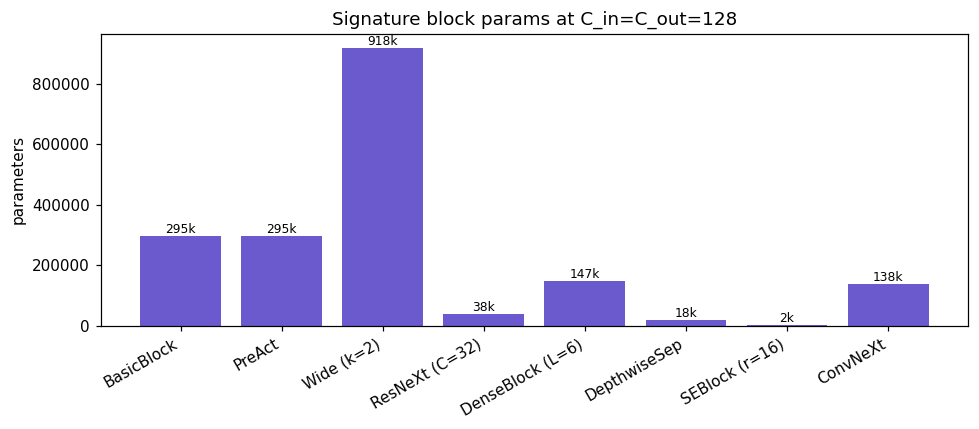
SEBlock (r=16)            2,184 params
DepthwiseSep             18,048 params
ResNeXt (C=32)           38,144 params
ConvNeXt                138,368 params
DenseBlock (L=6)        147,168 params
BasicBlock              295,424 params
PreAct                  295,424 params
Wide (k=2)              918,272 params
Key takeaways#
Pre-activation ResNet keeps the identity path clean (BN -> ReLU -> conv), improving gradient flow in very deep nets.
WideResNet trades depth for width \(k\); cost grows like \(k^2\), and width is more parallel-friendly.
ResNeXt adds cardinality via grouped convolutions: split-transform-merge with identical pathways, cheaper than full-width convs.
DenseNet concatenates all previous features (growth rate \(k\), channels \(C_{in}+Lk\)), maximizing reuse and parameter efficiency.
MobileNet factorizes convs into depthwise + pointwise, cutting cost to \(1/N + 1/k^2\); \(\alpha\) and \(\rho\) scale it further (\(\sim\alpha^2\), \(\sim\rho^2\)).
EfficientNet scales depth, width, and resolution jointly with \(\phi\) under \(\alpha\beta^2\gamma^2\approx2\), so FLOPs grow like \(2^{\phi}\).
SENet adds cheap channel attention (squeeze, excitation, scale) that recalibrates channels per input.
ConvNeXt modernizes ResNet with a patchify stem, large-kernel depthwise conv, inverted bottleneck, GELU, and LayerNorm.
Reading parameter and FLOP counts is the practical skill: it tells you where a block sits on the accuracy vs efficiency spectrum.
Further reading#
He, Zhang, Ren, Sun. Identity Mappings in Deep Residual Networks, 2016.
Huang, Liu, van der Maaten, Weinberger. Densely Connected Convolutional Networks (DenseNet), 2017.
Howard et al. MobileNets: Efficient Convolutional Neural Networks for Mobile Vision Applications, 2017.
Tan, Le. EfficientNet: Rethinking Model Scaling for Convolutional Neural Networks, 2019.
Hu, Shen, Sun. Squeeze-and-Excitation Networks (SENet), 2018.
Liu et al. A ConvNet for the 2020s (ConvNeXt), 2022.
Exercises#
Width costs quadratically. For a WideResNet block, measure parameters as the width multiplier \(k\) grows and confirm the growth is like \(k^2\).
Cardinality versus width. Build ResNeXt blocks at several cardinalities with matched parameter budgets. What does grouping buy at equal cost?
DenseNet channel arithmetic. Verify that the channel count after \(L\) layers is \(C_{in} + Lk\), and explain why concatenation rather than addition is what enables feature reuse.
Verify the depthwise saving. Measure the FLOP ratio of a depthwise-separable convolution against a standard one and check it against \(1/N + 1/k^2\).