📺 Lecture video  |  📄 Slides

Watch on YouTube

Week 4, Lecture 2: Why CNNs? Local Receptive Fields, Weight Sharing, Pooling, and Convolution Variants

NPTEL Deep Learning for Computer Vision | Prof. Vineeth N Balasubramanian, IIT Hyderabad

Companion notebook for §4.1 Introduction to CNNs.

What you will learn

• Why we move from handcrafted features (SIFT, LBP, HoG) to learned filters.

• Why flattening an image into a fully connected network (FNN) is wasteful and ignores 2D structure.

• The three core ideas that make CNNs work: local receptive fields, weight sharing, and pooling.

• How a tiny CNN condenses an image stage by stage.

• Useful convolution variants: dilated, transpose, depthwise-separable, and grouped convolution.

How to run

• Run the cells top to bottom. On Google Colab the interactive sliders work automatically.

• Each idea is shown first from scratch and then checked against the PyTorch built-in.

• Everything uses tiny synthetic tensors, so the whole notebook runs in a minute or two on CPU.

Contents

1. From handcrafted filters to learned filters

2. Why not just flatten the image into a fully connected network?

3. Idea 1: Local receptive fields (sparse connectivity)

4. Idea 2: Weight sharing (translation equivariance)

5. Idea 3: Pooling (parameter-free downsampling)

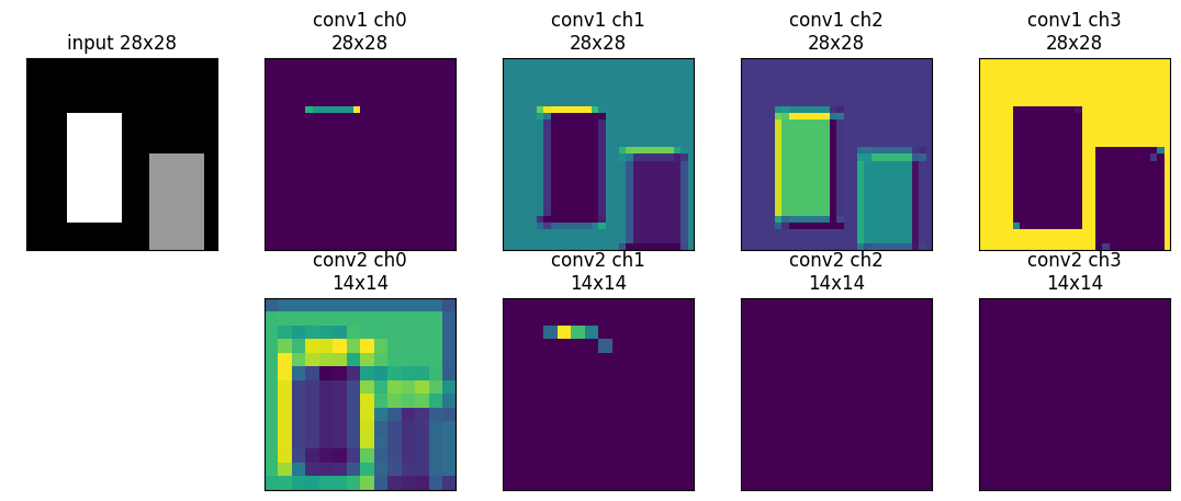
6. Putting it together: a tiny CNN

7. Convolution variants

Review

The previous lecture built the convolution operation and its hyperparameters, ending with the output-size formula \(W_2 = \frac{W_1 - F + 2P}{S} + 1\). This lecture takes those mechanics as given and asks why a convolutional layer is the right thing to put on an image.

Setup

Imports, inline plotting, seeds for reproducibility, and device selection (works on CPU and GPU).

import numpy as np
import torch
import torch.nn as nn
import torch.nn.functional as F
import matplotlib.pyplot as plt
%matplotlib inline
from ipywidgets import interact, IntSlider, Dropdown

torch.manual_seed(0)
np.random.seed(0)

device = torch.device('cuda' if torch.cuda.is_available() else 'cpu')
print('Using device:', device)
print('torch version:', torch.__version__)

Using device: cpu
torch version: 2.8.0

1. From handcrafted filters to learned filters

• Classic vision hand-designed features: SIFT, LBP, HoG. Effective, but a fixed, manual bottleneck.

• Key idea of CNNs: do not hand-pick the kernels. Treat the kernel entries as parameters and learn them by gradient descent, jointly with the classifier (backprop, covered next lecture).

• First we apply a fixed Sobel edge kernel to a synthetic shape (this is feature engineering).

• Then we train a single nn.Conv2d to reproduce that edge response and watch it become an edge detector.

# A small synthetic image with clear edges (no external files).
def make_shape_image(size=32):
    img = np.zeros((size, size), dtype=np.float32)
    img[8:24, 6:14] = 1.0    # a bright block
    img[14:28, 18:26] = 0.6  # a second, dimmer block -> more edges
    return img

img = make_shape_image(32)

# Fixed, handcrafted edge kernels (feature engineering).
sobel_x = torch.tensor([[-1., 0., 1.],
                        [-2., 0., 2.],
                        [-1., 0., 1.]])
sobel_y = torch.tensor([[-1., -2., -1.],
                        [ 0.,  0.,  0.],
                        [ 1.,  2.,  1.]])

x = torch.from_numpy(img)[None, None]                      # shape (1, 1, H, W)
resp_x = F.conv2d(x, sobel_x[None, None], padding=1)[0, 0]  # vertical edges
resp_y = F.conv2d(x, sobel_y[None, None], padding=1)[0, 0]  # horizontal edges

fig, axes = plt.subplots(1, 3, figsize=(10, 3.5))
axes[0].imshow(img, cmap='gray');          axes[0].set_title('synthetic image')
axes[1].imshow(resp_x, cmap='RdBu');       axes[1].set_title('Sobel-x (vertical edges)')
axes[2].imshow(resp_y, cmap='RdBu');       axes[2].set_title('Sobel-y (horizontal edges)')
for a in axes: a.axis('off')
plt.tight_layout(); plt.show()

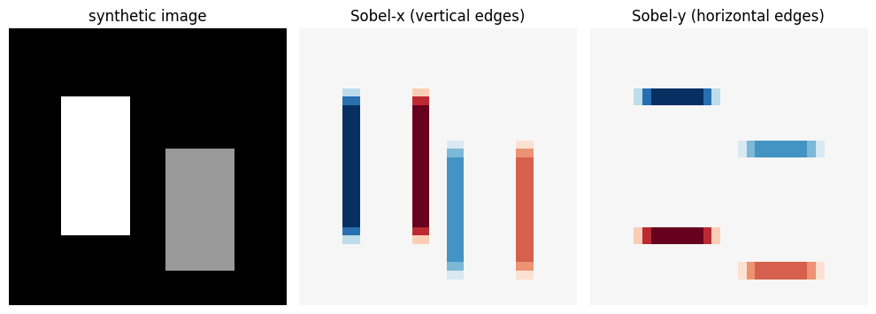
Now learn the filter. We feed random images to a single untrained nn.Conv2d and ask it to reproduce the output of the known Sobel-x kernel. Because the inputs are random, the 3x3 kernel is uniquely determined, so gradient descent should recover the edge detector itself.

# Build a supervised target: response of the known Sobel-x kernel on random images.
torch.manual_seed(0)
N = 64
train_imgs = torch.rand(N, 1, 16, 16)
target_kernel = sobel_x[None, None]
with torch.no_grad():
    targets = F.conv2d(train_imgs, target_kernel, padding=1)

# A single conv filter, randomly initialised.
conv = nn.Conv2d(1, 1, kernel_size=3, padding=1, bias=False)
kernel_before = conv.weight.detach().clone().squeeze().numpy()

conv = conv.to(device)
train_imgs_d, targets_d = train_imgs.to(device), targets.to(device)
opt = torch.optim.Adam(conv.parameters(), lr=0.08)

losses = []
for step in range(400):
    opt.zero_grad()
    loss = F.mse_loss(conv(train_imgs_d), targets_d)
    loss.backward()
    opt.step()
    losses.append(loss.item())

kernel_after = conv.weight.detach().cpu().squeeze().numpy()
print('final MSE loss:', round(losses[-1], 8))
print('max |learned - target|:', round(float(np.abs(kernel_after - sobel_x.numpy()).max()), 4))
print('learned kernel:\n', np.round(kernel_after, 2))
print('target  kernel:\n', sobel_x.numpy())

final MSE loss: 0.0
max |learned - target|: 0.0
learned kernel:
 [[-1.  0.  1.]
 [-2.  0.  2.]
 [-1.  0.  1.]]
target  kernel:
 [[-1.  0.  1.]
 [-2.  0.  2.]
 [-1.  0.  1.]]

# Visualise: kernel before vs after training, the target, and the loss curve.
vmax = np.abs(sobel_x.numpy()).max()
fig, axes = plt.subplots(1, 4, figsize=(12, 3.2))
axes[0].imshow(kernel_before, cmap='RdBu', vmin=-vmax, vmax=vmax); axes[0].set_title('kernel BEFORE\n(random init)')
axes[1].imshow(kernel_after,  cmap='RdBu', vmin=-vmax, vmax=vmax); axes[1].set_title('kernel AFTER\n(learned)')
axes[2].imshow(sobel_x.numpy(), cmap='RdBu', vmin=-vmax, vmax=vmax); axes[2].set_title('target\n(Sobel-x)')
for a in axes[:3]: a.set_xticks([]); a.set_yticks([])
axes[3].plot(losses); axes[3].set_yscale('log')
axes[3].set_title('training loss'); axes[3].set_xlabel('step'); axes[3].set_ylabel('MSE (log)')
plt.tight_layout(); plt.show()
print('The learned filter matched the handcrafted edge detector, discovered purely by gradient descent.')

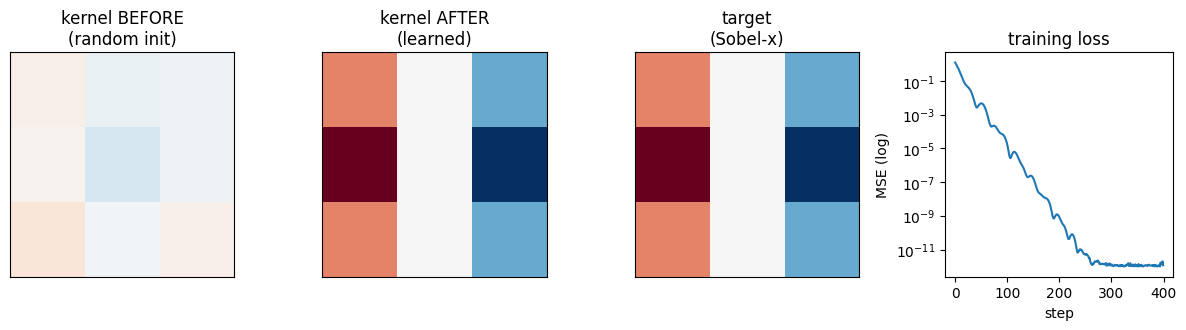
The learned filter matched the handcrafted edge detector, discovered purely by gradient descent.

2. Why not just flatten the image into a fully connected network?

• Flattening a \(28 \times 28\) image into a 784 vector throws away 2D structure: adjacent and far pixels are treated the same way.

• There is no natural way to reuse the same feature (for example an edge) at different locations.

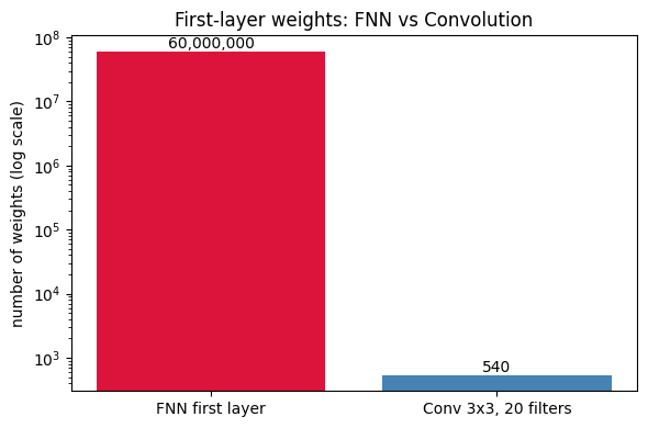
• Parameter blow-up: a 1 megapixel colour image (\(1000 \times 1000 \times 3\)) feeding 20 hidden units needs \(1000 \cdot 1000 \cdot 3 \cdot 20 = 60{,}000{,}000\) weights in the first layer alone.

• A convolution layer needs only \(K \times K \times C\) weights per filter, independent of image size.

# Reproduce the 60 million example from the slides.
def fnn_first_layer_weights(H, W, C, hidden):
    return H * W * C * hidden

def conv_layer_weights(K, C, filters):
    return K * K * C * filters

H, W, C, hidden = 1000, 1000, 3, 20      # 1 megapixel colour image, 20 hidden units
K, filters = 3, 20                        # a 3x3 conv layer with 20 filters
fnn = fnn_first_layer_weights(H, W, C, hidden)
conv_w = conv_layer_weights(K, C, filters)

print(f'FNN first-layer weights : {fnn:,}')
print(f'Conv (3x3, {filters} filters): {conv_w:,}')
print(f'FNN uses about {fnn // conv_w:,}x more weights than the conv layer.')

fig, ax = plt.subplots(figsize=(6, 4))
bars = ax.bar(['FNN first layer', 'Conv 3x3, 20 filters'], [fnn, conv_w],
              color=['crimson', 'steelblue'])
ax.set_yscale('log'); ax.set_ylabel('number of weights (log scale)')
ax.set_title('First-layer weights: FNN vs Convolution')
for b, v in zip(bars, [fnn, conv_w]):
    ax.text(b.get_x() + b.get_width()/2, v, f'{v:,}', ha='center', va='bottom')
plt.tight_layout(); plt.show()

FNN first-layer weights : 60,000,000
Conv (3x3, 20 filters): 540
FNN uses about 111,111x more weights than the conv layer.

Interactive calculator. Move the sliders for image height, width, channels, and hidden units. The FNN first-layer count is \(H \cdot W \cdot C \cdot \text{hidden}\); the conv count (\(K \times K \times C \times \text{filters}\), with \(K=3\)) barely moves because it does not depend on image size.

def show_param_explosion(H=1000, W=1000, C=3, hidden=20):
    K = 3
    fnn = H * W * C * hidden
    conv_w = K * K * C * hidden   # 'hidden' filters, for a fair comparison
    fig, ax = plt.subplots(figsize=(6, 4))
    bars = ax.bar([f'FNN ({H}x{W}x{C} -> {hidden})', f'Conv (3x3x{C}, {hidden} filters)'],
                  [fnn, conv_w], color=['crimson', 'steelblue'])
    ax.set_yscale('log'); ax.set_ylabel('weights (log scale)')
    ax.set_title(f'FNN {fnn:,}   vs   Conv {conv_w:,}')
    for b, v in zip(bars, [fnn, conv_w]):
        ax.text(b.get_x() + b.get_width()/2, v, f'{v:,}', ha='center', va='bottom')
    plt.tight_layout(); plt.show()

interact(show_param_explosion,
         H=IntSlider(min=28, max=2000, step=28, value=1000),
         W=IntSlider(min=28, max=2000, step=28, value=1000),
         C=IntSlider(min=1, max=3, step=1, value=3),
         hidden=IntSlider(min=1, max=100, step=1, value=20));

3. Idea 1: Local receptive fields (sparse connectivity)

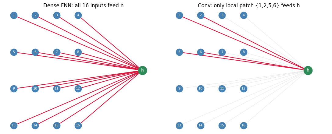
• Each hidden unit connects only to a small local patch of the input, not to every pixel.

• This captures local spatial relationships and slashes the parameter count.

• Slide example on a 4x4 input: only pixels 1, 2, 5, 6 feed the first hidden unit \(h_{11}\).

• Distant pixels are not lost: they interact indirectly through deeper layers, so the effective receptive field grows with depth.

# Compare dense (FNN) vs sparse (conv) connectivity into ONE hidden unit on a 4x4 input.
def draw_connectivity(ax, active_inputs, title, grid=4):
    pos = {}
    idx = 1
    for r in range(grid):
        for c in range(grid):
            pos[idx] = (c, grid - 1 - r)   # index 1..16, row-major
            idx += 1
    out_pos = (grid + 2, (grid - 1) / 2)
    for i, (px, py) in pos.items():
        on = i in active_inputs
        ax.plot([px, out_pos[0]], [py, out_pos[1]],
                color='crimson' if on else 'lightgray',
                lw=1.6 if on else 0.4, zorder=1)
    xs = [p[0] for p in pos.values()]; ys = [p[1] for p in pos.values()]
    ax.scatter(xs, ys, s=260, c='steelblue', zorder=2)
    for i, (px, py) in pos.items():
        ax.text(px, py, str(i), ha='center', va='center', color='white', fontsize=8, zorder=3)
    ax.scatter([out_pos[0]], [out_pos[1]], s=420, c='seagreen', zorder=2)
    ax.text(out_pos[0], out_pos[1], 'h', ha='center', va='center', color='white', zorder=3)
    ax.set_title(title); ax.axis('off'); ax.set_xlim(-0.5, grid + 3)

fig, axes = plt.subplots(1, 2, figsize=(11, 4.5))
draw_connectivity(axes[0], set(range(1, 17)), 'Dense FNN: all 16 inputs feed h')
draw_connectivity(axes[1], {1, 2, 5, 6},      'Conv: only local patch {1,2,5,6} feeds h')
plt.tight_layout(); plt.show()

Interactive receptive field. Pick an output unit of a conv layer (kernel size \(K\), stride 1) on a 4x4 input and see exactly which input pixels feed it.

def show_rf(out_row=0, out_col=0, K=2):
    grid = 4
    out_row = min(out_row, grid - K)   # clamp so the patch stays inside the image
    out_col = min(out_col, grid - K)
    highlight = np.zeros((grid, grid))
    highlight[out_row:out_row + K, out_col:out_col + K] = 1.0
    fig, ax = plt.subplots(figsize=(4.2, 4.2))
    ax.imshow(highlight, cmap='Reds', vmin=0, vmax=1)
    for r in range(grid):
        for c in range(grid):
            ax.text(c, r, str(r * grid + c + 1), ha='center', va='center',
                    color='black', fontsize=9)
    ax.set_xticks(range(grid)); ax.set_yticks(range(grid))
    ax.set_title(f'Output ({out_row},{out_col}) sees rows {out_row}-{out_row+K-1}, '
                 f'cols {out_col}-{out_col+K-1}\n({K*K} input pixels, not all 16)')
    plt.tight_layout(); plt.show()

interact(show_rf,
         out_row=IntSlider(min=0, max=2, step=1, value=0),
         out_col=IntSlider(min=0, max=2, step=1, value=0),
         K=IntSlider(min=2, max=3, step=1, value=2));

Depth grows the receptive field. Two highlighted pixels that do not interact in layer 1 still influence a shared unit deeper in the network. Stacking \(L\) layers of \(K \times K\) convolutions (stride 1) gives an effective receptive field of \(1 + L(K-1)\).

def rf_size(L, K=3):
    return 1 + L * (K - 1)

G, center = 9, 4
fig, axes = plt.subplots(1, 3, figsize=(10, 3.6))
for ax, L in zip(axes, [1, 2, 3]):
    half = rf_size(L) // 2
    m = np.zeros((G, G))
    m[center - half:center + half + 1, center - half:center + half + 1] = 1
    ax.imshow(m, cmap='Blues'); ax.axis('off')
    ax.set_title(f'{L} layer(s) of 3x3\neffective RF = {rf_size(L)}x{rf_size(L)}')
plt.tight_layout(); plt.show()
print('Distant pixels interact indirectly: the receptive field widens as we stack layers.')

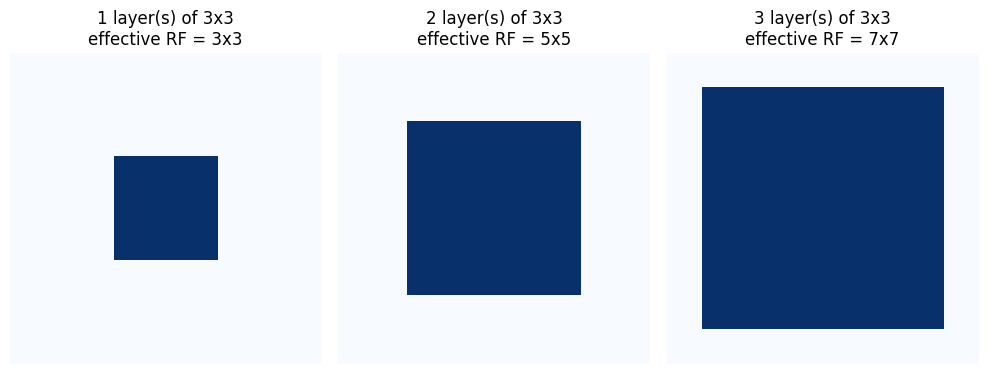
Distant pixels interact indirectly: the receptive field widens as we stack layers.

4. Idea 2: Weight sharing (translation equivariance)

• The same filter is slid across every location, so it detects a feature wherever it appears.

• This gives translation equivariance: shift the input and the response shifts the same way.

• One filter costs only \(K \times K\) weights no matter how large the image is.

• Use many filters to capture many kinds of features, each one applied everywhere.

# A small shape, shifted; the SAME filter gives a response that shifts with it.
def make_bar_image(size=24, row=10, col=4, w=4, h=4):
    im = np.zeros((size, size), dtype=np.float32)
    im[row:row + h, col:col + w] = 1.0
    return im

fig, axes = plt.subplots(2, 2, figsize=(7.5, 7))
for k, shift in enumerate([0, 10]):
    im = make_bar_image(col=4 + shift)
    r = F.conv2d(torch.from_numpy(im)[None, None], sobel_x[None, None], padding=1)[0, 0]
    axes[k, 0].imshow(im, cmap='gray');  axes[k, 0].set_title(f'input (shift={shift})')
    axes[k, 1].imshow(r, cmap='RdBu');   axes[k, 1].set_title('same filter response')
    for a in axes[k]: a.axis('off')
plt.tight_layout(); plt.show()
print('The filter responds identically to the shape, just moved: translation equivariance.')

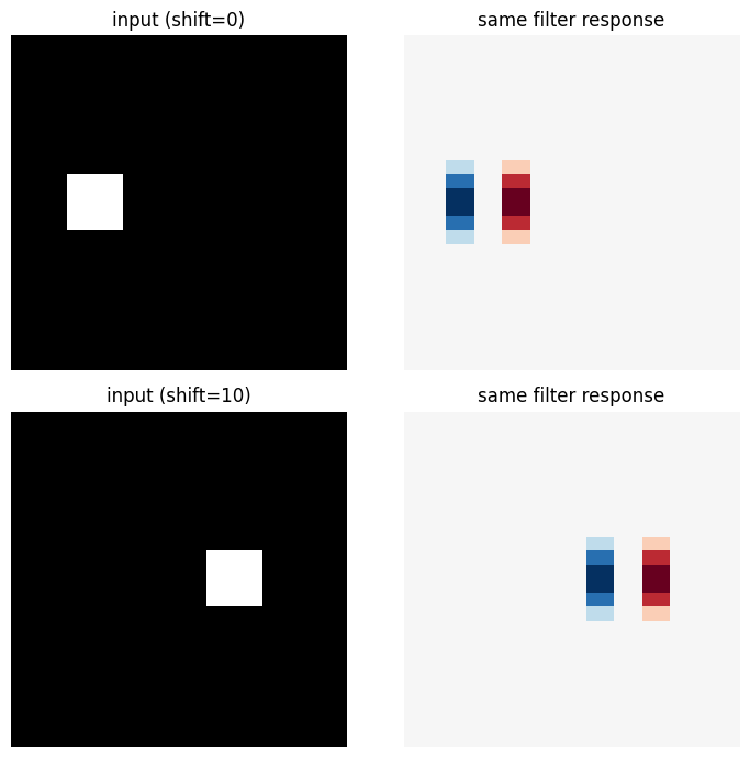
The filter responds identically to the shape, just moved: translation equivariance.

Interactive shift. Drag the shift slider and watch the input and its feature map move together because the SAME weights are used everywhere.

def show_shift(shift=0):
    im = make_bar_image(size=24, col=4 + shift)
    r = F.conv2d(torch.from_numpy(im)[None, None], sobel_x[None, None], padding=1)[0, 0]
    fig, axes = plt.subplots(1, 2, figsize=(8, 4))
    axes[0].imshow(im, cmap='gray'); axes[0].set_title(f'input (shift={shift})')
    axes[1].imshow(r, cmap='RdBu');  axes[1].set_title('feature map (shifts too)')
    for a in axes: a.axis('off')
    plt.tight_layout(); plt.show()

interact(show_shift, shift=IntSlider(min=0, max=14, step=1, value=0));

# With vs without weight sharing: parameter count for one 3x3 filter on a 28x28 input.
H = W = 28; K = 3
out_H = out_W = H - K + 1                     # 26x26 output positions
without_sharing = out_H * out_W * K * K       # a separate 3x3 kernel per position
with_sharing = K * K                          # one shared 3x3 kernel
print(f'Without weight sharing (locally connected): {without_sharing:,} weights')
print(f'With weight sharing (convolution):          {with_sharing} weights')
print(f'Weight sharing is about {without_sharing // with_sharing:,}x smaller here.')

Without weight sharing (locally connected): 6,084 weights
With weight sharing (convolution):          9 weights
Weight sharing is about 676x smaller here.

5. Idea 3: Pooling (parameter-free downsampling)

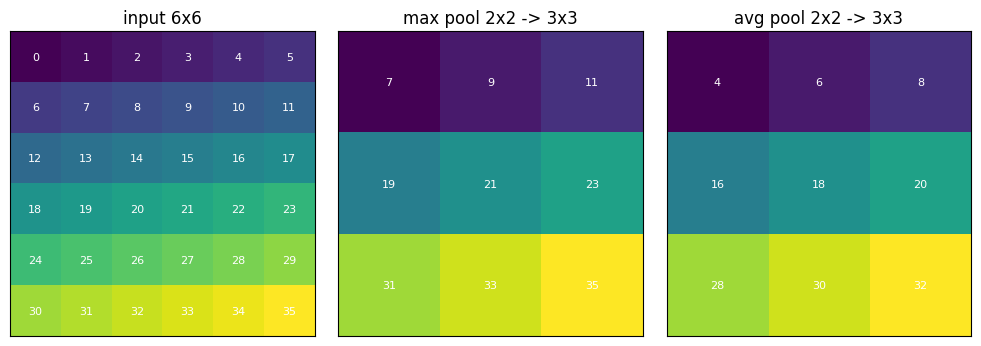
• Pooling condenses a feature map by summarizing each window with a single number.

• Common types: max, average, and L2 pooling. (Also mixed, spatial-pyramid, and spectral pooling, seen later.)

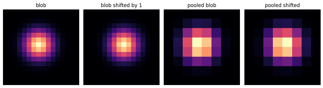
• It has no learnable parameters, adds robustness to small shifts, and shrinks maps to cut later compute.

• We implement max and average pooling with explicit loops, then confirm against the PyTorch built-ins.

def max_pool2d_scratch(x, k, s):
    H, W = x.shape
    out_H, out_W = (H - k) // s + 1, (W - k) // s + 1
    out = np.zeros((out_H, out_W), dtype=x.dtype)
    for i in range(out_H):
        for j in range(out_W):
            out[i, j] = x[i*s:i*s+k, j*s:j*s+k].max()
    return out

def avg_pool2d_scratch(x, k, s):
    H, W = x.shape
    out_H, out_W = (H - k) // s + 1, (W - k) // s + 1
    out = np.zeros((out_H, out_W), dtype=x.dtype)
    for i in range(out_H):
        for j in range(out_W):
            out[i, j] = x[i*s:i*s+k, j*s:j*s+k].mean()
    return out

m = np.arange(36, dtype=np.float32).reshape(6, 6)
mine_max = max_pool2d_scratch(m, 2, 2)
mine_avg = avg_pool2d_scratch(m, 2, 2)

t = torch.from_numpy(m)[None, None]
ref_max = F.max_pool2d(t, kernel_size=2, stride=2)[0, 0].numpy()
ref_avg = F.avg_pool2d(t, kernel_size=2, stride=2)[0, 0].numpy()

print('max pooling matches F.max_pool2d:', torch.allclose(torch.tensor(mine_max), torch.tensor(ref_max)))
print('avg pooling matches F.avg_pool2d:', torch.allclose(torch.tensor(mine_avg), torch.tensor(ref_avg)))

fig, axes = plt.subplots(1, 3, figsize=(10, 3.4))
for ax, data, title in zip(axes, [m, mine_max, mine_avg],
                           ['input 6x6', 'max pool 2x2 -> 3x3', 'avg pool 2x2 -> 3x3']):
    ax.imshow(data, cmap='viridis'); ax.set_title(title)
    for i in range(data.shape[0]):
        for j in range(data.shape[1]):
            ax.text(j, i, f'{data[i, j]:.0f}', ha='center', va='center', color='white', fontsize=8)
    ax.set_xticks([]); ax.set_yticks([])
plt.tight_layout(); plt.show()

max pooling matches F.max_pool2d: True
avg pooling matches F.avg_pool2d: True

Interactive pooling. Choose the pooling type and the window and stride. L2 pooling reports \(\sqrt{\sum x^2}\) over each window.

def show_pool(pool_type='max', k=2, s=2):
    rng = np.random.RandomState(0)
    m = rng.rand(8, 8).astype(np.float32)
    t = torch.from_numpy(m)[None, None]
    if pool_type == 'max':
        out = F.max_pool2d(t, kernel_size=k, stride=s)
    elif pool_type == 'avg':
        out = F.avg_pool2d(t, kernel_size=k, stride=s)
    else:  # L2 pooling: sqrt of the sum of squares in each window
        out = torch.sqrt(F.avg_pool2d(t**2, kernel_size=k, stride=s) * (k * k))
    out = out[0, 0].numpy()
    fig, axes = plt.subplots(1, 2, figsize=(8, 4))
    axes[0].imshow(m, cmap='viridis');  axes[0].set_title('input 8x8')
    axes[1].imshow(out, cmap='viridis'); axes[1].set_title(f'{pool_type} pool k={k}, s={s} -> {out.shape}')
    for a in axes: a.set_xticks([]); a.set_yticks([])
    plt.tight_layout(); plt.show()

interact(show_pool,
         pool_type=Dropdown(options=['max', 'avg', 'L2'], value='max'),
         k=IntSlider(min=1, max=4, step=1, value=2),
         s=IntSlider(min=1, max=4, step=1, value=2));

# Small-shift robustness: shift a blob by one pixel, then max pool. The pooled map barely changes.
yy, xx = np.mgrid[0:16, 0:16]
blob    = np.exp(-((xx - 7)**2 + (yy - 7)**2) / 8.0).astype(np.float32)
shifted = np.exp(-((xx - 8)**2 + (yy - 7)**2) / 8.0).astype(np.float32)   # moved right by 1

p1 = F.max_pool2d(torch.from_numpy(blob)[None, None],    kernel_size=2, stride=2)[0, 0].numpy()
p2 = F.max_pool2d(torch.from_numpy(shifted)[None, None], kernel_size=2, stride=2)[0, 0].numpy()
print('max abs difference between the two pooled maps:', round(float(np.abs(p1 - p2).max()), 4))

fig, axes = plt.subplots(1, 4, figsize=(11, 3))
for ax, d, t in zip(axes, [blob, shifted, p1, p2],
                    ['blob', 'blob shifted by 1', 'pooled blob', 'pooled shifted']):
    ax.imshow(d, cmap='magma'); ax.set_title(t); ax.axis('off')
plt.tight_layout(); plt.show()

max abs difference between the two pooled maps: 0.2819

6. Putting it together: a tiny CNN

• A typical CNN alternates convolution and pooling layers, then flattens into a classifier.

• Below: conv -> relu -> pool -> conv -> relu -> pool -> flatten -> fully connected.

• We print the tensor shape after every stage to watch the map condense, and visualize feature maps.

• The weights are randomly initialised (untrained), so we only inspect shapes and activations here.

torch.manual_seed(0)
conv1 = nn.Conv2d(1, 4, kernel_size=3, padding=1).to(device)
conv2 = nn.Conv2d(4, 8, kernel_size=3, padding=1).to(device)
fc    = nn.Linear(8 * 7 * 7, 10).to(device)

x = torch.from_numpy(make_shape_image(28))[None, None].to(device)
print('input           ', tuple(x.shape))
a1 = F.relu(conv1(x));            print('after conv1+relu', tuple(a1.shape))
p1 = F.max_pool2d(a1, 2);         print('after pool1     ', tuple(p1.shape))
a2 = F.relu(conv2(p1));           print('after conv2+relu', tuple(a2.shape))
p2 = F.max_pool2d(a2, 2);         print('after pool2     ', tuple(p2.shape))
flat = p2.flatten(1);             print('after flatten   ', tuple(flat.shape))
logits = fc(flat);                print('logits          ', tuple(logits.shape))

input            (1, 1, 28, 28)
after conv1+relu (1, 4, 28, 28)
after pool1      (1, 4, 14, 14)
after conv2+relu (1, 8, 14, 14)
after pool2      (1, 8, 7, 7)
after flatten    (1, 392)
logits           (1, 10)

# Visualise how the spatial maps shrink while the number of channels grows.
a1n = a1.detach().cpu()[0]
a2n = a2.detach().cpu()[0]
fig, axes = plt.subplots(2, 5, figsize=(11, 4.6))
axes[0, 0].imshow(x.detach().cpu()[0, 0], cmap='gray'); axes[0, 0].set_title('input 28x28')
for c in range(4):
    axes[0, c + 1].imshow(a1n[c], cmap='viridis'); axes[0, c + 1].set_title(f'conv1 ch{c}\n28x28')
axes[1, 0].axis('off')
for c in range(4):
    axes[1, c + 1].imshow(a2n[c], cmap='viridis'); axes[1, c + 1].set_title(f'conv2 ch{c}\n14x14')
for a in axes.ravel(): a.set_xticks([]); a.set_yticks([])
plt.tight_layout(); plt.show()

7. Convolution variants

A few practical relatives of the standard convolution.

7a. Dilated convolution

• Adds a dilation rate \(d\) that spaces out the kernel taps. Dilation 1 is standard convolution.

• It enlarges the receptive field without subsampling, which is the subtle difference from stride greater than 1.

• Stride greater than 1 skips output positions and shrinks the map; dilation keeps stride 1 and keeps the resolution while seeing a wider area. A \(K \times K\) kernel with dilation \(d\) has an effective size \(d(K-1)+1\).

def dilated_footprint(K=3, d=1, size=9):
    m = np.zeros((size, size))
    center = size // 2
    start = center - (d * (K - 1)) // 2
    for i in range(K):
        for j in range(K):
            m[start + i*d, start + j*d] = 1.0
    return m

fig, axes = plt.subplots(1, 3, figsize=(10, 3.6))
for ax, d in zip(axes, [1, 2, 3]):
    ax.imshow(dilated_footprint(3, d, 9), cmap='Oranges')
    eff = d * 2 + 1
    ax.set_title(f'3x3 kernel, dilation={d}\neffective RF = {eff}x{eff}'); ax.axis('off')
plt.tight_layout(); plt.show()

# Confirm receptive field and output size with the real layer (stride 1, no padding).
for d in [1, 2, 3]:
    out = nn.Conv2d(1, 1, kernel_size=3, dilation=d)(torch.zeros(1, 1, 16, 16))
    print(f'dilation={d}: effective kernel {d*2+1}x{d*2+1}, '
          f'input 16x16 -> output {tuple(out.shape[2:])} (stride stays 1, map stays large)')

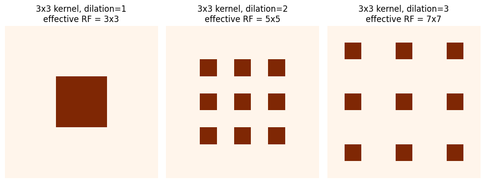
dilation=1: effective kernel 3x3, input 16x16 -> output (14, 14) (stride stays 1, map stays large)
dilation=2: effective kernel 5x5, input 16x16 -> output (12, 12) (stride stays 1, map stays large)
dilation=3: effective kernel 7x7, input 16x16 -> output (10, 10) (stride stays 1, map stays large)

Interactive dilation. Slide the dilation rate and watch the kernel footprint spread out over the grid.

def show_dilation(d=2):
    fig, ax = plt.subplots(figsize=(4.2, 4.2))
    ax.imshow(dilated_footprint(3, d, 9), cmap='Oranges')
    eff = d * 2 + 1
    ax.set_title(f'3x3 kernel, dilation={d}, effective RF = {eff}x{eff}')
    ax.set_xticks(range(9)); ax.set_yticks(range(9))
    plt.tight_layout(); plt.show()

interact(show_dilation, d=IntSlider(min=1, max=3, step=1, value=2));

7b. Transpose convolution

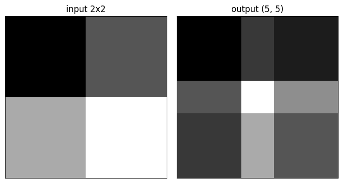
• Learnable upsampling. Also called deconvolution (a poor name) or upconvolution.

• Instead of a fixed interpolation rule, the network learns how to fill in the upsampled values.

• Output size grows as \(H_{out} = (H_{in} - 1)\cdot S - 2P + K\).

# Upsample a 2x2 input to a larger map with a learnable transpose conv.
inp = torch.tensor([[1., 2.], [3., 4.]])[None, None]
deconv = nn.ConvTranspose2d(1, 1, kernel_size=3, stride=2, bias=False)
with torch.no_grad():
    deconv.weight.fill_(1.0)   # fixed weights just to make the pattern visible
out = deconv(inp)
print('input 2x2 -> output', tuple(out.shape[2:]), '(learnable upsampling)')

fig, axes = plt.subplots(1, 2, figsize=(7, 3.6))
axes[0].imshow(inp[0, 0].numpy(), cmap='gray'); axes[0].set_title('input 2x2')
axes[1].imshow(out[0, 0].detach().numpy(), cmap='gray'); axes[1].set_title(f'output {tuple(out.shape[2:])}')
for a in axes: a.set_xticks([]); a.set_yticks([])
plt.tight_layout(); plt.show()

input 2x2 -> output (5, 5) (learnable upsampling)

Interactive transpose convolution. Increase the stride to upsample more; padding crops the border. Watch the output size grow.

def show_transpose(stride=2, padding=0):
    inp = torch.ones(1, 1, 4, 4)
    deconv = nn.ConvTranspose2d(1, 1, kernel_size=3, stride=stride, padding=padding, bias=False)
    with torch.no_grad():
        deconv.weight.fill_(1.0)
    out = deconv(inp)
    fig, axes = plt.subplots(1, 2, figsize=(8, 4))
    axes[0].imshow(inp[0, 0].numpy(), cmap='gray'); axes[0].set_title('input 4x4')
    axes[1].imshow(out[0, 0].detach().numpy(), cmap='gray')
    axes[1].set_title(f'stride={stride}, padding={padding} -> {tuple(out.shape[2:])}')
    for a in axes: a.set_xticks([]); a.set_yticks([])
    plt.tight_layout(); plt.show()

interact(show_transpose,
         stride=IntSlider(min=1, max=3, step=1, value=2),
         padding=IntSlider(min=0, max=2, step=1, value=0));

7c. Depthwise-separable and grouped convolution

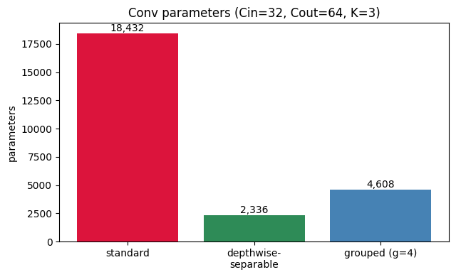
• Depthwise-separable = a per-channel depthwise conv followed by a 1x1 pointwise conv. Far fewer parameters.

• Grouped convolution splits the channels into \(g\) groups, dividing the parameter count by \(g\).

• Below we count parameters for the same shapes and verify against real nn.Conv2d modules.

Cin, Cout, K, g = 32, 64, 3, 4

standard  = Cin * Cout * K * K
depthwise = Cin * K * K            # one KxK kernel per input channel
pointwise = Cin * Cout             # 1x1 conv mixing channels
dw_sep    = depthwise + pointwise
grouped   = (Cin // g) * (Cout // g) * K * K * g   # = standard / g

# Verify the hand counts against real PyTorch layers.
n = lambda mod: sum(p.numel() for p in mod.parameters())
assert n(nn.Conv2d(Cin, Cout, K, bias=False)) == standard
assert n(nn.Conv2d(Cin, Cin, K, groups=Cin, bias=False)) + n(nn.Conv2d(Cin, Cout, 1, bias=False)) == dw_sep
assert n(nn.Conv2d(Cin, Cout, K, groups=g, bias=False)) == grouped
print(f'standard             : {standard:,}')
print(f'depthwise-separable  : {dw_sep:,}  ({standard / dw_sep:.1f}x fewer)')
print(f'grouped (g={g})        : {grouped:,}  ({standard / grouped:.0f}x fewer)')

fig, ax = plt.subplots(figsize=(6.5, 4))
labels = ['standard', 'depthwise-\nseparable', f'grouped (g={g})']
vals = [standard, dw_sep, grouped]
bars = ax.bar(labels, vals, color=['crimson', 'seagreen', 'steelblue'])
ax.set_ylabel('parameters'); ax.set_title(f'Conv parameters (Cin={Cin}, Cout={Cout}, K={K})')
for b, v in zip(bars, vals):
    ax.text(b.get_x() + b.get_width()/2, v, f'{v:,}', ha='center', va='bottom')
plt.tight_layout(); plt.show()

standard             : 18,432
depthwise-separable  : 2,336  (7.9x fewer)
grouped (g=4)        : 4,608  (4x fewer)

Key takeaways

• Handcrafted features (SIFT, LBP, HoG) work but are a manual bottleneck. CNNs learn the filters instead, via backprop.

• Flattening images into an FNN ignores 2D structure, cannot reuse features across locations, and explodes in parameters (the 60 million example).

• Local receptive fields: each unit sees a local patch. Sparse connectivity, far fewer parameters, and distant pixels still interact through depth.

• Weight sharing: one filter reused everywhere gives translation equivariance and only \(K \times K\) weights per filter.

• Pooling: parameter-free downsampling (max, average, L2) that aggregates information, adds small-shift robustness, and shrinks maps.

• A typical CNN alternates convolution and pooling, then flattens into a classifier.

• Variants: dilated (wider receptive field, no subsampling), transpose (learnable upsampling), depthwise-separable and grouped (parameter savings).

Exercises

• In the FNN calculator, push the image size up and watch the FNN weights explode while the conv count stays flat.

• Change the learned-filter target to sobel_y and see the kernel it recovers.

• In the pooling widget, compare max vs average vs L2 and vary the window and stride.

• In the dilated widget, confirm the effective receptive field is \(d(K-1)+1\).

• In the transpose widget, find settings that upsample a 4x4 input to 8x8 or larger.

Open question (teaser for the backprop lecture): max pooling only passes the maximum value forward, so is it differentiable, and how do we backpropagate through it? We answer this in the next notebook.