
📺 Lecture video | 📄 Slides
Week 3, Lecture 5: Momentum and Nesterov Accelerated Gradient#
NPTEL Deep Learning for Computer Vision | Prof. Vineeth N Balasubramanian, IIT Hyderabad
Companion notebook for §3.3 Gradient Descent and Variants.
Plain gradient descent (GD) can be painfully slow on the twisty, non-convex error surfaces of real networks. This notebook builds two classic fixes from scratch, momentum and Nesterov accelerated gradient (NAG), on a small library of 2D loss surfaces so you can literally watch them move.
What you will learn
A zoo of 2D loss surfaces (an ill-conditioned “ravine”, a saddle, a double well, and a plateau), each a plain function that returns its value and its analytic gradient. These stand in for the local minima, saddle points, and flat regions of real networks.
Vanilla GD from scratch and why it zig-zags across a ravine while crawling slowly along its floor.
Momentum from scratch: the velocity update \(v_t = \gamma v_{t-1} + \alpha \nabla\), which “builds speed in consistent directions”, damps the oscillation, and reaches the minimum much faster (though it overshoots).
Nesterov (NAG) from scratch: the “look before you leap” gradient at the look-ahead point, which trims the overshoot.
A check that our from-scratch momentum matches
torch.optim.SGD(momentum=...)exactly.Three interactive widgets to explore surfaces, learning rate, \(\gamma\), and step count.
How to run Everything is tiny 2D math and runs in a few seconds on Colab CPU or GPU (no GPU needed). Run the setup cell first, then go top to bottom.
Contents
A zoo of 2D loss surfaces (value and analytic gradient)
Vanilla gradient descent from scratch
Momentum from scratch
Nesterov accelerated gradient (NAG) from scratch
Setup#
# Run this cell first. Works on Colab (CPU or GPU) and local Jupyter.
import sys, subprocess
# ipywidgets ships with Colab; install only if it is missing.
try:
    import ipywidgets  # noqa: F401
except ImportError:
    subprocess.run([sys.executable, "-m", "pip", "install", "-q", "ipywidgets"])

import numpy as np
import torch
import torch.nn as nn
import torch.nn.functional as F
import matplotlib.pyplot as plt
from ipywidgets import interact, interactive, FloatSlider, IntSlider, Dropdown, Checkbox, fixed
%matplotlib inline

# Reproducibility
torch.manual_seed(0)
np.random.seed(0)

# Use a GPU if one is available, otherwise CPU. Every demo here is tiny and
# runs in seconds on CPU, so no GPU is required.
device = torch.device("cuda" if torch.cuda.is_available() else "cpu")

plt.rcParams["figure.figsize"] = (7, 4.5)
plt.rcParams["axes.grid"] = True
plt.rcParams["axes.axisbelow"] = True

print("PyTorch", torch.__version__, "| device:", device)
PyTorch 2.8.0 | device: cpu
Review#
Gradient descent finds a minimum of a differentiable cost \(J(\theta)\) by pushing the parameters \(\theta\) downhill, opposite the gradient:
where \(\alpha\) is the learning rate. A key property to keep in mind:
The update is proportional to the gradient. So steps are large where the gradient is large (steep walls) and small where the gradient is small (shallow, flat regions).
That single fact causes trouble on the error surfaces of real networks, which are non-convex. Three features hurt GD:
Local minima: unlike a convex bowl with one global minimum, deep nets have many local minima.
Saddle points: the gradient is (near) zero, yet it is not a minimum (a max along one direction, a min along another). They are rare in low dimensions but become very common in high dimensions, and they give a false impression of convergence.
Plateaus / flat regions: the gradient is tiny, so GD takes tiny steps and crawls for a long time. Raising \(\alpha\) speeds this up but risks divergence on the steep parts.
In this notebook we build small 2D surfaces that isolate each of these, then watch GD, momentum, and NAG traverse them. We treat the two parameters as coordinates \(x\) and \(y\) (two entries of \(\theta\)), so a trajectory is a path on a contour map.
1. A zoo of 2D loss surfaces (value and analytic gradient)#
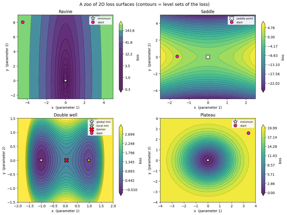
We start bottom-up. Each surface is a plain function \(f(x, y)\) paired with its closed-form gradient \(\nabla f(x, y)\), so no autograd is needed and everything is fast. The four surfaces and the phenomenon each one illustrates:
Ravine (ill-conditioned quadratic) \(f = \tfrac{1}{2}(a x^2 + b y^2)\) with \(a \gg b\). Steep in \(x\), nearly flat in \(y\): contours are long thin ellipses. This is the classic oscillation / zig-zag trap.
Saddle \(f = x^2 - y^2\). A minimum along \(x\), a maximum along \(y\); the gradient vanishes at the origin even though it is not a minimum.
Double well \(f = (x^2 - 1)^2 + y^2 + c\,x\). Two minima separated by a barrier, so there is a global minimum and a local one (the tilt \(c\,x\) makes the left well deeper).
Plateau \(f = C\,\big(1 - e^{-(x^2 + y^2)/(2 w^2)}\big)\). A single minimum at the origin surrounded by a wide flat region where the gradient nearly vanishes.
We also finite-difference-check every analytic gradient so we can trust them.
class Surface:
    """A 2D loss surface: value f(x,y), analytic grad(x,y), plus a cached mesh
    for fast contour redraws inside widgets."""
    def __init__(self, name, f, grad, xlim, ylim, start, markers, level_kind, res=161):
        self.name = name
        self.f = f                      # f(x, y): works on scalars OR numpy arrays
        self.grad = grad                # grad(x, y): scalars -> np.array([gx, gy])
        self.xlim, self.ylim = xlim, ylim
        self.start = np.array(start, dtype=float)
        self.markers = markers          # list of (x, y, label, color, marker)
        xs = np.linspace(xlim[0], xlim[1], res)
        ys = np.linspace(ylim[0], ylim[1], res)
        self.XX, self.YY = np.meshgrid(xs, ys)
        self.ZZ = f(self.XX, self.YY)
        zmin, zmax = float(self.ZZ.min()), float(self.ZZ.max())
        if level_kind == "geom":        # long-range quadratic: geometric levels
            self.levels = np.geomspace(0.3, zmax, 12)
        elif level_kind == "well":      # zoom the levels near the two wells
            self.levels = np.linspace(-0.16, 3.0, 22)
        else:                           # plain linear levels
            self.levels = np.linspace(zmin, zmax, 22)

    def loss(self, p):
        return float(self.f(p[0], p[1]))


# ---- (a) Ravine: ill-conditioned quadratic, steep in x, shallow in y ----
A_RAV, B_RAV = 20.0, 0.4
def ravine_f(x, y): return 0.5 * (A_RAV * x**2 + B_RAV * y**2)
def ravine_grad(x, y): return np.array([A_RAV * x, B_RAV * y])

# ---- (b) Saddle: min along x, max along y ----
def saddle_f(x, y): return x**2 - y**2
def saddle_grad(x, y): return np.array([2.0 * x, -2.0 * y])

# ---- (c) Double well: two minima + a barrier, slightly tilted ----
TILT = 0.15
def well_f(x, y): return (x**2 - 1.0)**2 + y**2 + TILT * x
def well_grad(x, y): return np.array([4.0 * x * (x**2 - 1.0) + TILT, 2.0 * y])
# Stationary points on the x-axis solve 4x^3 - 4x + TILT = 0 (two minima, one max).
_roots = np.sort(np.roots([4.0, 0.0, -4.0, TILT]).real)
WELL_L, WELL_BAR, WELL_R = _roots[0], _roots[1], _roots[2]

# ---- (d) Plateau: single min at origin, flat far away ----
C_PLAT, W_PLAT = 20.0, 1.4
def plateau_f(x, y): return C_PLAT * (1.0 - np.exp(-(x**2 + y**2) / (2.0 * W_PLAT**2)))
def plateau_grad(x, y):
    e = np.exp(-(x**2 + y**2) / (2.0 * W_PLAT**2))
    return np.array([C_PLAT * e * x / W_PLAT**2, C_PLAT * e * y / W_PLAT**2])

SURFACES = {
    "Ravine": Surface("Ravine", ravine_f, ravine_grad, (-5, 5), (-2.5, 9), (-4.5, 8.0),
                      [(0, 0, "minimum", "white", "*")], "geom"),
    "Saddle": Surface("Saddle", saddle_f, saddle_grad, (-2.5, 2.5), (-5, 5), (-1.6, 0.05),
                      [(0, 0, "saddle point", "white", "X")], "lin"),
    "Double well": Surface("Double well", well_f, well_grad, (-2, 2), (-1.5, 1.5), (1.3, 1.0),
                           [(WELL_L, 0, "global min", "white", "*"),
                            (WELL_R, 0, "local min", "gold", "*"),
                            (WELL_BAR, 0, "barrier", "red", "X")], "well"),
    "Plateau": Surface("Plateau", plateau_f, plateau_grad, (-4, 4), (-4, 4), (3.4, 2.6),
                       [(0, 0, "minimum", "white", "*")], "lin"),
}

# Compare each analytic gradient to a central finite difference.
def fd_grad(f, x, y, h=1e-5):
    gx = (f(x + h, y) - f(x - h, y)) / (2 * h)
    gy = (f(x, y + h) - f(x, y - h)) / (2 * h)
    return np.array([gx, gy])

print("finite-difference check of the analytic gradients (max abs error):")
for name, s in SURFACES.items():
    px, py = 0.7, -0.5
    err = np.abs(s.grad(px, py) - fd_grad(s.f, px, py)).max()
    print(f"  {name:12s}: {err:.2e}")
print("\ndouble-well stationary x:", np.round(_roots, 3),
      " (outer two are minima, middle is the barrier)")
finite-difference check of the analytic gradients (max abs error):
  Ravine      : 4.15e-11
  Saddle      : 6.93e-12
  Double well : 2.90e-10
  Plateau     : 1.16e-10

double-well stationary x: [-1.018  0.038  0.981]  (outer two are minima, middle is the barrier)
def plot_surface(surface, ax, show_cbar=False):
    """Filled + line contours of a surface on ax, with its special points marked."""
    cs = ax.contourf(surface.XX, surface.YY, surface.ZZ, levels=surface.levels,
                     cmap="viridis", alpha=0.85, extend="both")
    ax.contour(surface.XX, surface.YY, surface.ZZ, levels=surface.levels,
               colors="k", linewidths=0.4, alpha=0.5)
    for (mx, my, label, color, marker) in surface.markers:
        ax.plot([mx], [my], marker=marker, color=color, markersize=13,
                markeredgecolor="k", linestyle="None", label=label)
    ax.set_xlim(*surface.xlim)
    ax.set_ylim(*surface.ylim)
    ax.set_xlabel("x  (parameter 1)")
    ax.set_ylabel("y  (parameter 2)")
    ax.grid(False)
    if show_cbar:
        plt.colorbar(cs, ax=ax, shrink=0.85, label="loss")
    return cs


# Draw all four surfaces so the phenomena are visible side by side.
fig, axes = plt.subplots(2, 2, figsize=(12, 9))
for ax, (name, s) in zip(axes.ravel(), SURFACES.items()):
    plot_surface(s, ax, show_cbar=True)
    ax.plot([s.start[0]], [s.start[1]], marker="o", color="deeppink",
            markersize=9, markeredgecolor="k", linestyle="None", label="start")
    ax.set_title(f"{name}")
    ax.legend(loc="upper right", fontsize=8, framealpha=0.9)
fig.suptitle("A zoo of 2D loss surfaces (contours = level sets of the loss)",
             fontsize=13)
plt.tight_layout()
plt.show()
2. Vanilla gradient descent from scratch#
The update is just one line: at the current point evaluate the gradient and step against it,
We put all three optimizers in a single run_optimizer(surface, method, ...) so
we can reuse it. For now only the "gd" branch matters; we add the "momentum"
and "nesterov" branches in the next parts (same function, one extra line each).
Watch the ravine. Because the step is proportional to the gradient, GD takes big steps across the steep \(x\) walls (so it overshoots and zig-zags from wall to wall) but tiny steps along the shallow \(y\) floor (so it crawls toward the minimum). The result is a slow, oscillating descent.
def run_optimizer(surface, method="gd", lr=0.06, gamma=0.9, steps=60, start=None):
    """Run one of {gd, momentum, nesterov} on a surface from a start point.

    Returns (path, losses):
      path   : array of shape (steps + 1, 2), the visited points.
      losses : array of shape (steps + 1,), the loss at each point.

    Update rules (matching the lecture slides, alpha = lr, gamma = momentum):
      GD        : theta <- theta - alpha * grad(theta)
      Momentum  : v <- gamma * v + alpha * grad(theta) ;            theta <- theta - v
      Nesterov  : v <- gamma * v + alpha * grad(theta - gamma * v); theta <- theta - v
    """
    p = surface.start.copy() if start is None else np.array(start, dtype=float)
    v = np.zeros(2)
    path, losses = [p.copy()], [surface.loss(p)]
    for _ in range(steps):
        if method == "gd":
            g = surface.grad(p[0], p[1])
            p = p - lr * g
        elif method == "momentum":
            g = surface.grad(p[0], p[1])
            v = gamma * v + lr * g
            p = p - v
        elif method == "nesterov":
            look = p - gamma * v                       # look before you leap
            g = surface.grad(look[0], look[1])
            v = gamma * v + lr * g
            p = p - v
        else:
            raise ValueError("unknown method: " + str(method))
        p = np.clip(p, -1e4, 1e4)                       # keep everything finite if lr is huge
        path.append(p.copy())
        losses.append(surface.loss(p))
    return np.array(path), np.array(losses)


METHOD_LABEL = {"gd": "Gradient Descent", "momentum": "Momentum", "nesterov": "Nesterov (NAG)"}
METHOD_COLOR = {"gd": "tab:red", "momentum": "tab:blue", "nesterov": "tab:green"}


def plot_path(ax, path, color, label, marker="o"):
    """Overlay a trajectory (with a big dot at the start) on a contour axis."""
    ax.plot(path[:, 0], path[:, 1], color=color, marker=marker, markersize=3,
            linewidth=1.6, alpha=0.9, label=label)
    ax.plot([path[0, 0]], [path[0, 1]], marker="o", color=color, markersize=9,
            markeredgecolor="k")


print("run_optimizer and plot helpers are ready.")
run_optimizer and plot helpers are ready.
# Vanilla GD on the ravine.
ravine = SURFACES["Ravine"]
LR, GAMMA, STEPS = 0.06, 0.9, 60
gd_path, gd_loss = run_optimizer(ravine, method="gd", lr=LR, steps=STEPS)

fig, (ax1, ax2) = plt.subplots(1, 2, figsize=(12, 4.8))
plot_surface(ravine, ax1)
plot_path(ax1, gd_path, METHOD_COLOR["gd"], "GD path")
ax1.set_title(f"Vanilla GD zig-zags across the ravine (lr = {LR})")
ax1.legend(loc="upper right", fontsize=8)

ax2.plot(gd_loss, color=METHOD_COLOR["gd"], marker="o", markersize=2, label="GD")
ax2.set_xlabel("step")
ax2.set_ylabel("loss")
ax2.set_title(f"GD loss vs step (final loss = {gd_loss[-1]:.3f})")
ax2.legend(loc="upper right")
plt.tight_layout()
plt.show()

print("After", STEPS, "steps GD is still at loss", round(float(gd_loss[-1]), 3),
      "and y =", round(float(gd_path[-1, 1]), 3), "(the minimum is at y = 0).")
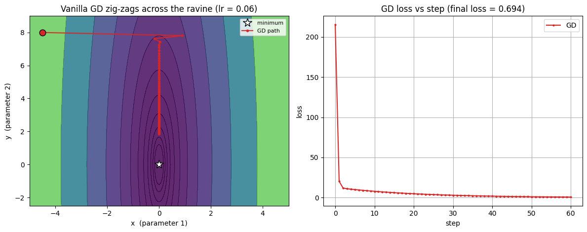
After 60 steps GD is still at loss 0.694 and y = 1.862 (the minimum is at y = 0).
3. Momentum from scratch#
Intuition (from the slide): build speed in consistent directions. A heavy ball rolling downhill keeps some of its previous velocity, so it accelerates where the gradient keeps pointing the same way and averages out directions that keep flipping. Concretely we keep a velocity \(v\) and update:
\(\gamma \in [0, 1)\) is the momentum coefficient (how much past velocity carries over). Larger \(\gamma\) means the past matters more. Practitioners often start at \(\gamma = 0.5\) and raise it to \(0.9\) or higher once learning stabilizes.
Along the steep \(x\) walls the gradient keeps flipping sign, so the velocity terms partly cancel: momentum damps the oscillation (high-curvature direction).
Along the shallow \(y\) floor the gradient is consistent, so velocity accumulates: momentum gets a larger effective step (low-curvature direction) and races to the minimum.
The catch: it builds so much speed along the floor that it overshoots the minimum and oscillates around it before settling. Even so, it reaches the minimum far faster than vanilla GD.
# Momentum on the ravine, overlaid against vanilla GD.
mom_path, mom_loss = run_optimizer(ravine, method="momentum", lr=LR, gamma=GAMMA, steps=STEPS)

fig, (ax1, ax2) = plt.subplots(1, 2, figsize=(12, 4.8))
plot_surface(ravine, ax1)
plot_path(ax1, gd_path, METHOD_COLOR["gd"], "GD")
plot_path(ax1, mom_path, METHOD_COLOR["momentum"], "Momentum")
ax1.set_title(f"Momentum damps the zig-zag and races down the floor (gamma = {GAMMA})")
ax1.legend(loc="upper right", fontsize=8)

ax2.plot(gd_loss, color=METHOD_COLOR["gd"], label="GD")
ax2.plot(mom_loss, color=METHOD_COLOR["momentum"], label="Momentum")
ax2.set_xlabel("step")
ax2.set_ylabel("loss")
ax2.set_title("loss vs step: momentum drops faster but overshoots")
ax2.legend(loc="upper right")
plt.tight_layout()
plt.show()

print("lowest y reached by momentum:", round(float(mom_path[:, 1].min()), 3),
      "(it overshoots past the minimum at y = 0 and swings back)")
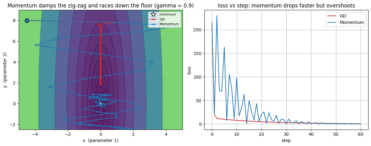
lowest y reached by momentum: -2.661 (it overshoots past the minimum at y = 0 and swings back)
Our momentum equals torch.optim.SGD(momentum=...)#
PyTorch’s SGD writes the update with the learning rate outside the velocity,
\(b_t = \gamma b_{t-1} + g_t,\ \theta \leftarrow \theta - \alpha b_t\). That is
algebraically the same as our \(v_t = \gamma v_{t-1} + \alpha g_t\) with \(v_t = \alpha b_t\).
To prove it, we feed our analytic gradients into a real torch.optim.SGD
optimizer (respecting device) and check the trajectories match to machine
precision.
# Drive a real torch optimizer with our analytic gradients and compare paths.
def run_torch_sgd(surface, lr, gamma, steps, nesterov=False):
    param = nn.Parameter(torch.tensor(surface.start, dtype=torch.float64, device=device))
    opt = torch.optim.SGD([param], lr=lr, momentum=gamma, nesterov=nesterov)
    path = [param.detach().cpu().numpy().copy()]
    for _ in range(steps):
        g = surface.grad(float(param[0]), float(param[1]))
        param.grad = torch.tensor(g, dtype=torch.float64, device=device)
        opt.step()
        path.append(param.detach().cpu().numpy().copy())
    return np.array(path)

torch_mom_path = run_torch_sgd(ravine, LR, GAMMA, STEPS, nesterov=False)
max_diff = np.abs(mom_path - torch_mom_path).max()
print("max |from-scratch momentum  -  torch.optim.SGD(momentum)| =", f"{max_diff:.2e}")
print("They agree:", bool(max_diff < 1e-9))
print("\nNote: torch's nesterov=True is an algebraically reformulated NAG that")
print("measures the gradient at the current iterate. It captures the same look-")
print("ahead idea and lands in essentially the same place, but its intermediate")
print("iterates are indexed differently, so it will not match our look-ahead")
print("version step for step. We keep the slide's look-ahead form below.")
max |from-scratch momentum  -  torch.optim.SGD(momentum)| = 1.78e-15
They agree: True

Note: torch's nesterov=True is an algebraically reformulated NAG that
measures the gradient at the current iterate. It captures the same look-
ahead idea and lands in essentially the same place, but its intermediate
iterates are indexed differently, so it will not match our look-ahead
version step for step. We keep the slide's look-ahead form below.
/var/folders/j0/z7mrqrv9121_0pm8njw3pbxh0000gp/T/ipykernel_41736/3001247675.py:7: UserWarning: Converting a tensor with requires_grad=True to a scalar may lead to unexpected behavior.
Consider using tensor.detach() first. (Triggered internally at .../work/pytorch/pytorch/pytorch/torch/csrc/autograd/generated/python_variable_methods.cpp:836.)
  g = surface.grad(float(param[0]), float(param[1]))
4. Nesterov accelerated gradient (NAG) from scratch#
Key idea (from the slide): look before you leap. Momentum is about to move by \(\gamma v_{t-1}\) no matter what, so why not evaluate the gradient there, at the look-ahead point \(\theta_t - \gamma v_{t-1}\), instead of where we are now? That gives the gradient a chance to brake early if the look-ahead point is already climbing back up the other side of the valley:
The only change from momentum is where the gradient is measured (at the look-ahead point, not the current point). Empirically this reduces the overshoot and converges a bit faster. Below we overlay all three on the ravine.
# All three optimizers on the ravine from the same start.
nag_path, nag_loss = run_optimizer(ravine, method="nesterov", lr=LR, gamma=GAMMA, steps=STEPS)

fig, (ax1, ax2) = plt.subplots(1, 2, figsize=(12, 4.8))
plot_surface(ravine, ax1)
plot_path(ax1, gd_path, METHOD_COLOR["gd"], "GD")
plot_path(ax1, mom_path, METHOD_COLOR["momentum"], "Momentum")
plot_path(ax1, nag_path, METHOD_COLOR["nesterov"], "Nesterov (NAG)")
ax1.set_title("GD vs Momentum vs NAG on the ravine")
ax1.legend(loc="upper right", fontsize=8)

ax2.plot(gd_loss, color=METHOD_COLOR["gd"], label="GD")
ax2.plot(mom_loss, color=METHOD_COLOR["momentum"], label="Momentum")
ax2.plot(nag_loss, color=METHOD_COLOR["nesterov"], label="Nesterov (NAG)")
ax2.set_xlabel("step")
ax2.set_ylabel("loss")
ax2.set_title("loss vs step (lower is better)")
ax2.legend(loc="upper right")
plt.tight_layout()
plt.show()

print("lowest y reached (how far each overshoots the minimum at y = 0):")
print(f"  Momentum : {mom_path[:, 1].min():+.3f}")
print(f"  NAG      : {nag_path[:, 1].min():+.3f}   (smaller overshoot)")
print("final loss:  GD =", round(float(gd_loss[-1]), 4),
      "| Momentum =", round(float(mom_loss[-1]), 4),
      "| NAG =", round(float(nag_loss[-1]), 4))
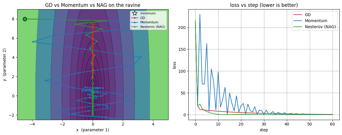
lowest y reached (how far each overshoots the minimum at y = 0):
  Momentum : -2.661
  NAG      : -1.997   (smaller overshoot)
final loss:  GD = 0.6937 | Momentum = 0.513 | NAG = 0.0019
Interactive explorations#
Three widgets. Each callback does the full computation and redraws, so they run at their default values with no manual interaction needed.
Widget 1: pick a surface, optimizer, learning rate, and momentum#
Choose any of the four surfaces and any optimizer, then move the learning-rate and \(\gamma\) sliders. Watch how the trajectory changes. Some things to try:
On the Ravine, raise
lrtoward the top of its range with Nesterov selected: it eventually diverges (NAG has a tighter stability limit than momentum). This is the “raise the learning rate and risk divergence” warning from the plateau slide.On the Plateau, compare
Gradient Descent(creeps) againstMomentum(builds speed and crosses the flat region).On the Saddle, watch how quickly each method escapes the flat neighbourhood of the origin.
def explore(surface_name="Ravine", method="momentum", lr=0.06, gamma=0.9):
    surf = SURFACES[surface_name]
    path, losses = run_optimizer(surf, method=method, lr=lr, gamma=gamma, steps=60)
    fig, (ax1, ax2) = plt.subplots(1, 2, figsize=(12, 4.8))
    plot_surface(surf, ax1)
    plot_path(ax1, path, METHOD_COLOR[method], METHOD_LABEL[method])
    ax1.set_title(f"{METHOD_LABEL[method]} on {surface_name}\n"
                  f"lr = {lr:.3f}, gamma = {gamma:.2f}, final loss = {losses[-1]:.4f}")
    ax1.legend(loc="upper right", fontsize=8)
    ax2.plot(losses, color=METHOD_COLOR[method], marker="o", markersize=2)
    ax2.set_xlabel("step")
    ax2.set_ylabel("loss")
    ax2.set_title("loss vs step")
    plt.tight_layout()
    plt.show()


interact(explore,
         surface_name=Dropdown(options=list(SURFACES.keys()), value="Ravine",
                               description="surface"),
         method=Dropdown(options=[("Gradient Descent", "gd"), ("Momentum", "momentum"),
                                  ("Nesterov (NAG)", "nesterov")],
                         value="momentum", description="method"),
         lr=FloatSlider(min=0.005, max=0.12, step=0.005, value=0.06,
                        description="lr", readout_format=".3f"),
         gamma=FloatSlider(min=0.0, max=0.98, step=0.02, value=0.9, description="gamma"));
Widget 2: step through GD vs Momentum vs NAG side by side#
The three full trajectories on the ravine are precomputed once; the slider just
reveals more of each path. Slide steps up from 1 and watch GD still oscillating
its way down while Momentum and NAG have already reached the floor, with NAG
hugging the valley more tightly than Momentum.
# Precompute the full paths ONCE, then the widget just indexes into them.
MAXSTEP = 60
_res = {m: run_optimizer(ravine, method=m, lr=LR, gamma=GAMMA, steps=MAXSTEP)
        for m in ("gd", "momentum", "nesterov")}


def compare_steps(step=15):
    fig, axes = plt.subplots(1, 3, figsize=(15, 4.6))
    for ax, m in zip(axes, ("gd", "momentum", "nesterov")):
        path, losses = _res[m]
        plot_surface(ravine, ax)
        plot_path(ax, path[:step + 1], METHOD_COLOR[m], METHOD_LABEL[m])
        ax.set_title(f"{METHOD_LABEL[m]}\nstep {step}, loss = {losses[step]:.3f}")
        ax.legend(loc="upper right", fontsize=7)
    fig.suptitle("Same ravine, same start: how far each optimizer has gotten", fontsize=12)
    plt.tight_layout()
    plt.show()


interact(compare_steps, step=IntSlider(min=1, max=MAXSTEP, step=1, value=15, description="steps"));
Widget 3: how \(\gamma\) controls damping and overshoot#
Fix the ravine and the learning rate, and sweep the momentum coefficient \(\gamma\).
At \(\gamma = 0\) both momentum and NAG reduce to plain GD (the three curves coincide).
As \(\gamma\) grows the descent along the floor speeds up, but Momentum starts to overshoot the minimum and loop around it.
NAG’s look-ahead keeps its overshoot smaller than Momentum’s at the same \(\gamma\).
Push \(\gamma\) toward \(0.98\) to see the oscillations grow large (too much momentum).
def gamma_demo(gamma=0.9):
    pg, lg = run_optimizer(ravine, method="gd", lr=LR, steps=60)          # gamma has no effect
    pm, lm = run_optimizer(ravine, method="momentum", lr=LR, gamma=gamma, steps=60)
    pn, ln = run_optimizer(ravine, method="nesterov", lr=LR, gamma=gamma, steps=60)

    fig, (ax1, ax2) = plt.subplots(1, 2, figsize=(12, 4.8))
    plot_surface(ravine, ax1)
    plot_path(ax1, pm, METHOD_COLOR["momentum"], "Momentum")
    plot_path(ax1, pn, METHOD_COLOR["nesterov"], "Nesterov (NAG)")
    ax1.set_title(f"Momentum vs NAG on the ravine, gamma = {gamma:.2f}")
    ax1.legend(loc="upper right", fontsize=8)

    ax2.plot(lg, color=METHOD_COLOR["gd"], label="GD (no momentum)")
    ax2.plot(lm, color=METHOD_COLOR["momentum"], label="Momentum")
    ax2.plot(ln, color=METHOD_COLOR["nesterov"], label="Nesterov (NAG)")
    ax2.set_xlabel("step")
    ax2.set_ylabel("loss")
    ax2.set_title(f"loss vs step  (Momentum overshoot to y = {pm[:, 1].min():+.2f})")
    ax2.legend(loc="upper right")
    plt.tight_layout()
    plt.show()


interact(gamma_demo,
         gamma=FloatSlider(min=0.0, max=0.98, step=0.02, value=0.9, description="gamma"));
Key takeaways#
GD steps are proportional to the gradient, so on an ill-conditioned ravine it takes big steps across the steep walls (zig-zag) and tiny steps along the shallow floor (slow). Non-convex surfaces add local minima, saddle points, and plateaus that make plain GD slow or stuck.
Momentum keeps a velocity \(v_t = \gamma v_{t-1} + \alpha \nabla\) and steps by \(\theta \leftarrow \theta - v_t\). It damps oscillation in high-curvature directions and accelerates in consistent, low-curvature directions. It reaches the minimum much faster than GD, but it overshoots and oscillates before settling. Typical \(\gamma\): start at \(0.5\), raise to \(0.9\) or higher.
Nesterov (NAG) measures the gradient at the look-ahead point \(\theta_t - \gamma v_{t-1}\) (“look before you leap”), which lets it brake early and trim the overshoot. Empirically it is a bit faster than plain momentum.
Our from-scratch momentum matches
torch.optim.SGD(momentum=...)exactly; the whole optimizer is just that one velocity line.
Exercises#
Escaping a saddle or plateau. In Widget 1 pick the Saddle (or Plateau) and compare
Gradient DescentagainstMomentum. Does the accumulated velocity carry the ball through the near-flat region faster? Why does a consistent (even if tiny) gradient help momentum here?Crossing a barrier. On the Double well, start is in the shallower (local) well. Raise \(\gamma\) toward \(0.99\) in Widget 1: can enough momentum roll the ball over the barrier into the deeper global minimum? What does that suggest, and what is the risk of using such a large \(\gamma\) everywhere (revisit Widget 3)?
Stability. On the Ravine with Nesterov, increase
lruntil it diverges, then compare the threshold to Momentum. Which one tolerates the larger learning rate?